
Training course in data analysis for genomic surveillance of African malaria vectors
Workshop 7 - Gene flow and the spread of insecticide resistance
Module 3 - Investigating gene flow at loci of interest using haplotype clustering#
Theme: Analysis
In the previous module of workshop 7, we saw how selective sweeps can be shared between populations through adaptive gene flow. When we find loci of interest like this, where we have evidence that gene flow is occuring, we may want to investigate in more detail. We may want to know how many different haplotypes are under selection (i.e. how many independent selective sweeps are there). We may also want to know how far these haplotypes have spread, both in geographical space and between species. To answer these questions, we can analyse the similarity of our haplotypes with haplotype clustering.
Learning objectives#
Explain why we want to perform haplotype clustering.
Understand what a dendrogram is and what it displays.
Use haplotype clustering to investigate genomic regions with evidence of adaptive gene flow.
Lecture#
English#
Français#
Please note that the code in the cells below might differ from that shown in the video. This can happen because Python packages and their dependencies change due to updates, necessitating tweaks to the code.
Setup#
Install and import the packages we’ll need.
%pip install -q --no-warn-conflicts malariagen_data
Note that authentication is required to access data through the package, please follow the instructions here.
import malariagen_data
# Import libraries
import numpy as np
import scipy.cluster
import matplotlib.pyplot as plt
import string
import plotly.io as pio
pio.renderers.default = "notebook+colab"

def dendrogram(
    haplotypes,
    linkage_method='single',
    metric='hamming',
    orient='right',
    size=(7,5)
):
    """Takes a 2D numpy array of values and performs hierarchical clustering
    and plots dendrogram."""

    # perform clustering
    linkage_matrix = scipy.cluster.hierarchy.linkage(
        haplotypes,
        method=linkage_method,
        metric=metric
    )
    if metric == 'hamming':
        # convert hamming to number of snp differences
        linkage_matrix[:,2] *= haplotypes.shape[1]

    # plot a dendrogram
    figsize = size if orient == 'right' else size[::-1]
    fig, ax = plt.subplots(figsize=size)
    z = scipy.cluster.hierarchy.dendrogram(
        linkage_matrix,
        orientation=orient,
        leaf_rotation=0 if orient=='right' else 90,
        # label leaf nodes using letters
        labels=[' '.join(map(str, row)) + " | " + str(letter)
                for letter, row in zip(string.ascii_uppercase, haplotypes)],
        ax=ax
    )

    # tidy up the plot
    if orient == "right":
        ax.set_xlabel("Distance (no. SNPs)")
        ax.set_ylabel("Haplotypes")
        # change the limit so we can easily see identical haplotypes
        ax.set_xlim(-0.05, np.max(z['dcoord']) + 0.2)
    else:
        ax.set_xlabel("Haplotypes")
        ax.set_ylabel("Distance (no. SNPs)")
        # change the limit so we can easily see identical haplotypes
        ax.set_ylim(-0.05, np.max(z['dcoord']) + 0.2)
Introduction to hierarchical clustering#
Clustering is the task of grouping a set of objects in such a way that objects in the same group (called a cluster) are more similar to each other than to those in other groups. It is widely-used across a vast array of fields, and there are many different algorithms and approaches to perform clustering.
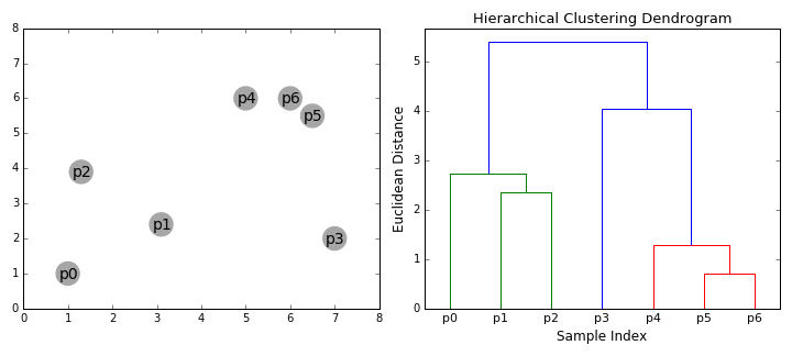
In this module we will use one approach, called hierarchical clustering. In hierarchical clustering, the algorithms typically begin with every data point in its own cluster, and then pairs of data points or clusters are merged moving up the hierarchy. The order in which we merge two points is based on their distance (smallest distance first). We can visualise this clustering with dendrograms, which provide us with a visual interpretation of the hierarchical relationship between variables.
The below animation shows this clustering process both in 2D space (left), and moving up the dendrogram hierarchy (right). We can see that we begin by grouping the two closest data points first, and continue iteratively until all data points are in one cluster, at which point, the dendrogram is complete. Here, the sample indices correspond to the dendrogram leaves.
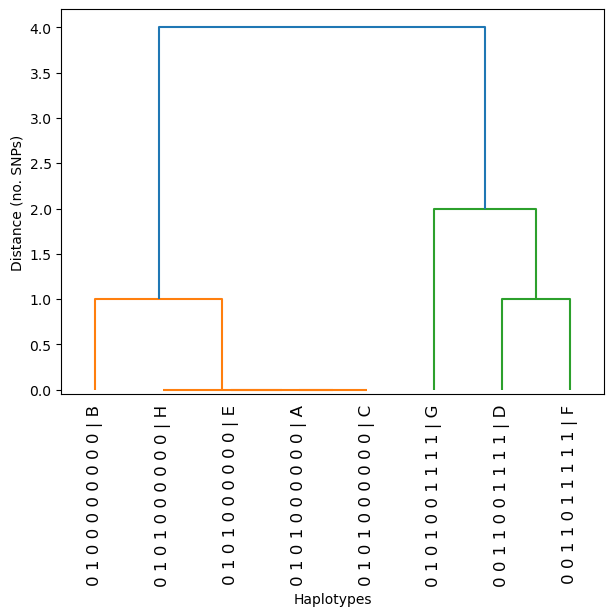
To gain some intuition for both hierarchical clustering and dendrograms, we’ll create some artificial ‘haplotypes’, and cluster them in the same way that we would when performing analyses.
haplotypes = np.array(
    [[0, 1, 0, 1, 0, 0, 0, 0, 0, 0],  # hap A
     [0, 1, 0, 0, 0, 0, 0, 0, 0, 0],  # hap B
     [0, 1, 0, 1, 0, 0, 0, 0, 0, 0],  # hap C
     [0, 0, 1, 1, 0, 0, 1, 1, 1, 1],  # hap D
     [0, 1, 0, 1, 0, 0, 0, 0, 0, 0],  # hap E
     [0, 0, 1, 1, 0, 1, 1, 1, 1, 1],  # hap F
     [0, 1, 0, 1, 0, 0, 1, 1, 1, 1],  # hap G
     [0, 1, 0, 1, 0, 0, 0, 0, 0, 0]],  # hap H
)

haplotypes.shape
(8, 10)
There are 8 haplotypes, and each haplotype contains 10 SNPs, though some of the SNPs are invariant. We can probably tell just by looking, that some haplotypes in this array look quite similar to each other.
We will label the dendrogram leaves with the haplotype ID (A-H) and its sequence, and perform hierarchical clustering to see how the clustering algorithm is working.
dendrogram(haplotypes, metric='hamming', linkage_method='single', orient='right')
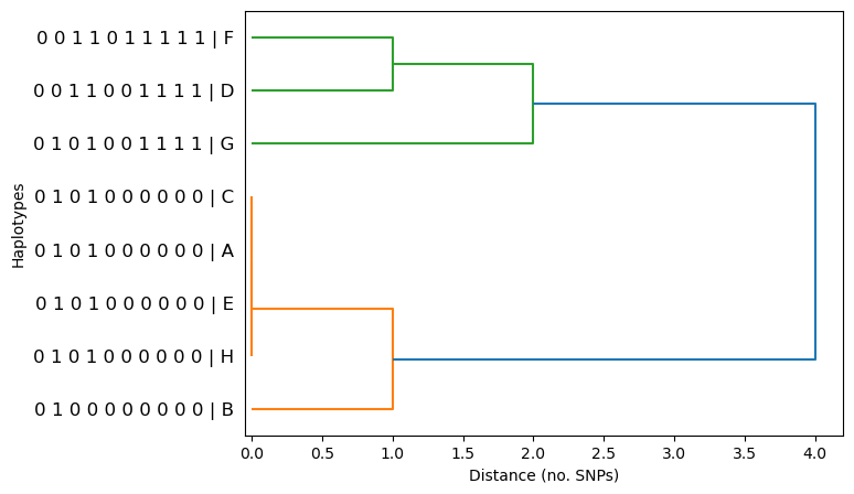
When looking for selective sweeps in dendrograms, we are looking for large clusters of identical or very closely related haplotypes. We can see that the algorithm is grouping similar haplotypes together (i.e. clustering). We can also see there are 4 haplotypes (C,A,E,H) which are identical to each other. By looking at the x-axes, the distance between haplotypes in SNPs, we can discern how closely related haplotypes are. For example, haplotype B is 1 SNP away from the four identical haplotypes (C,A,E,H).
When we perform hiearchical clustering we must specify the distance metric, which is how we calculate the distance between data points, or in our case haplotypes. For haplotype analysis, we use something called hamming distance, shown below.

The Hamming distance between two equal-length vectors is the number of positions at which the corresponding values are different. In the case of haplotypes, it is the proportion of SNPs on the haplotype that differ. We can multiply this value by the total number of SNPs, to get a distance which corresponds to the total number of SNP differences.
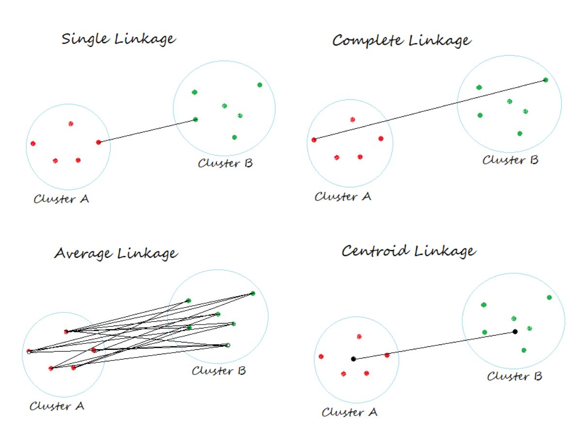
We must also specify a linkage method. This parameter determines how we calculate the distance between clusters at each stage of the clustering process. See the below image. The distance for single linkage takes the shortest distance between any pair of between cluster data points, whereas complete linkage takes the longest possible distance.
Lets take a look at this using our artificial haplotypes…
dendrogram(haplotypes, linkage_method='single', metric='hamming', orient='right')
In the above plot, haplotype G and (F,D) have a distance between them of 2 SNPs. This is because haplotype G differs from haplotype D by 2 SNPs, but differs from haplotype F by 3 SNPs. As we are using single linkage, the shortest distance (2 SNPs) is used as the distance between the clusters.
Lets see what happens if we use complete linkage.
dendrogram(haplotypes, linkage_method='complete', metric='hamming', orient='right')
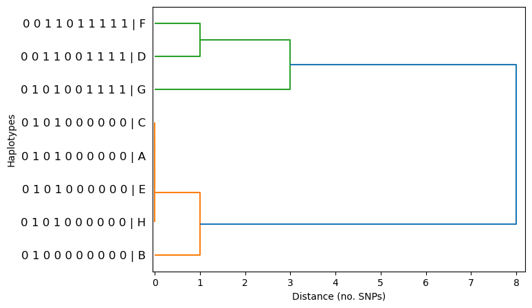
Now we can see that the distance at that position is now 3 SNPs, which is what we would expect - it’s now the maximum distance between cluster members. If we compare the orange and green clusters, we can also see that the overall distance between them has changed from 4 SNPs to 8 SNPs. Thats because the four identical orange haplotypes (C,A,E,H) only differ from haplotype G by 4 SNPs, whereas haplotype B differs haplotype F by 8 SNPs!
It’s important to note that in practice, however, the exact choice of linkage method will not have much affect on the overall dendrogram shape, or on our conclusions. This is because we are looking for large clusters of identical or near-identical haplotypes, and they will appear similar regardless of the linkage method. Therefore, it’s quite fine to stick with the default - single linkage.
Lets see the same plot again, but this time change the orientation. This is how we will view the dendrogram when analying our Anopheles gambiae haplotypes.
dendrogram(haplotypes, linkage_method='single', metric='hamming', orient='top')
When we look at a region of the genome under selection, we should see clusters of haplotypes that look highly similar to each other. Patterns like the four identical haplotypes may be indicative of a selective sweep, where a beneficial mutation has arisen and spread through a population. The spread of the beneficial allele also causes nearby linked mutations to spread with it, through hitchhiking - because the nearby alleles are in close physical proximity, they are inherited together. This means that when you look in a specific genomic region under selection, haplotypes which have the same selective sweep will appear as highly similar or identical. This signature is captured by genome-wide selection scans, for example, H12.
When we perform haplotype clustering in An. gambiae s.l, the procedure is exactly as above, the only difference being that rather than haplotypes 10 SNPs long, we use much larger windows of haplotypes.
Haplotype clustering#
Lets first configure access to the MalariaGEN Ag3 data resource.
ag3 = malariagen_data.Ag3()
ag3
| MalariaGEN Ag3 API client | |
|---|---|
| Please note that data are subject to terms of use, for more information see the MalariaGEN website or contact support@malariagen.net. See also the Ag3 API docs. | |
| Storage URL | gs://vo_agam_release_master_us_central1 |
| Data releases available | 3.0, 3.1, 3.2, 3.3, 3.4, 3.5, 3.6, 3.7, 3.8, 3.9, 3.10, 3.11, 3.12, 3.13, 3.14 |
| Results cache | None |
| Cohorts analysis | 20250131 |
| AIM analysis | 20220528 |
| Site filters analysis | dt_20200416 |
| Software version | malariagen_data 15.2.0 |
| Client location | Iowa, United States (Google Cloud us-central1) |
For this module we introduce a new function ag3.plot_haplotype_clustering(). This function produces an interactive dendrogram with plotly, which allows us to hover over leaves and retrieve information about each haplotype, such as its species, or the country and sample set it belongs to. We can also colour the leaves and control their shape with the use of the color and symbol parameters. Lets take a look at the help for this function…
?ag3.plot_haplotype_clustering
Signature:
ag3.plot_haplotype_clustering(
    region: Union[str, malariagen_data.util.Region, Mapping, List[Union[str, malariagen_data.util.Region, Mapping]], Tuple[Union[str, malariagen_data.util.Region, Mapping], ...]],
    analysis: str = 'default',
    sample_sets: Union[str, Sequence[str], NoneType] = None,
    sample_query: Optional[str] = None,
    sample_query_options: Optional[dict] = None,
    cohort_size: Optional[int] = None,
    random_seed: int = 42,
    color: Union[str, Mapping, NoneType] = None,
    symbol: Union[str, Mapping, NoneType] = None,
    linkage_method: Literal['single', 'complete', 'average', 'weighted', 'centroid', 'median', 'ward'] = 'single',
    count_sort: Optional[bool] = None,
    distance_sort: Optional[bool] = None,
    title: Union[str, bool, NoneType] = True,
    title_font_size: int = 14,
    width: Optional[int] = None,
    height: Optional[int] = 500,
    show: bool = True,
    renderer: Optional[str] = None,
    render_mode: Literal['auto', 'svg', 'webgl'] = 'svg',
    leaf_y: int = 0,
    marker_size: Union[int, float] = 5,
    line_width: Union[int, float] = 0.5,
    line_color: str = 'black',
    color_discrete_sequence: Optional[List] = None,
    color_discrete_map: Optional[Mapping] = None,
    category_orders: Union[List, Mapping, NoneType] = None,
    legend_sizing: Literal['constant', 'trace'] = 'constant',
    chunks: Union[int, str, Tuple[Union[int, str], ...], Callable[[Tuple[int, ...]], Union[int, str, Tuple[Union[int, str], ...]]]] = 'native',
    inline_array: bool = True,
) -> Optional[plotly.graph_objs._figure.Figure]
Docstring:
Hierarchically cluster haplotypes in region and produce an interactive
plot.

Parameters
----------
region : str or Region or Mapping or list of str or Region or Mapping or tuple of str or Region or Mapping
    Region of the reference genome. Can be a contig name, region string
    (formatted like "{contig}:{start}-{end}"), or identifier of a genome
    feature such as a gene or transcript. Can also be a sequence (e.g.,
    list) of regions.
analysis : str, optional, default: 'default'
    Which haplotype phasing analysis to use. See the
    `phasing_analysis_ids` property for available values.
sample_sets : sequence of str or str or None, optional
    List of sample sets and/or releases. Can also be a single sample set
    or release.
sample_query : str or None, optional
    A pandas query string to be evaluated against the sample metadata, to
    select samples to be included in the returned data.
sample_query_options : dict or None, optional
    A dictionary of arguments that will be passed through to pandas
    query() or eval(), e.g. parser, engine, local_dict, global_dict,
    resolvers.
cohort_size : int or None, optional
    Randomly down-sample to this value if the number of samples in the
    cohort is greater. Raise an error if the number of samples is less
    than this value.
random_seed : int, optional, default: 42
    Random seed used for reproducible down-sampling.
color : str or Mapping or None, optional
    Name of variable to use to color the markers.
symbol : str or Mapping or None, optional
    Name of the variable to use to choose marker symbols.
linkage_method : {'single', 'complete', 'average', 'weighted', 'centroid', 'median', 'ward'}, optional, default: 'single'
    The linkage algorithm to use. See the Linkage Methods section of the
    scipy.cluster.hierarchy.linkage docs for full descriptions.
count_sort : bool or None, optional
    If True, for each node n, the child with the minimum number of
    descendants is plotted first. Note distance_sort and count_sort cannot
    both be True.
distance_sort : bool or None, optional
    If True, for each node n, if True, the child with the minimum distance
    between is plotted first. Note distance_sort and count_sort cannot
    both be True.
title : str or bool or None, optional, default: True
    If True, attempt to use metadata from input dataset as a plot title.
    Otherwise, use supplied value as a title.
title_font_size : int, optional, default: 14
    Font size for the plot title.
width : int or None, optional
    Figure width in pixels (px).
height : int or None, optional, default: 500
    Figure height in pixels (px).
show : bool, optional, default: True
    If true, show the plot. If False, do not show the plot, but return the
    figure.
renderer : str or None, optional
    The name of the renderer to use.
render_mode : {'auto', 'svg', 'webgl'}, optional, default: 'svg'
    The type of rendering backend to use. See also
    https://plotly.com/python/webgl-vs-svg/.
leaf_y : int, optional, default: 0
    Y coordinate at which to plot the leaf markers.
marker_size : int or float, optional, default: 5
    Marker size.
line_width : int or float, optional, default: 0.5
    Line width.
line_color : str, optional, default: 'black'
    Line color.
color_discrete_sequence : List or None, optional
    Provide a list of colours to use.
color_discrete_map : Mapping or None, optional
    Provide an explicit mapping from values to colours.
category_orders : List or Mapping or None, optional
    Control the order in which values appear in the legend.
legend_sizing : {'constant', 'trace'}, optional, default: 'constant'
    Determines if the legend items symbols scale with their corresponding
    "trace" attributes or remain "constant" independent of the symbol size
    on the graph.
chunks : int or str or tuple of int or str or Callable[[typing.Tuple[int, ...]], int or str or tuple of int or str], optional, default: 'native'
    Define how input data being read from zarr should be divided into
    chunks for a dask computation. If 'native', use underlying zarr
    chunks. If a string specifying a target memory size, e.g., '300 MiB',
    resize chunks in arrays with more than one dimension to match this
    size. If 'auto', let dask decide chunk size.  If 'ndauto', let dask
    decide chunk size but only for arrays with more than one dimension. If
    'ndauto0', as 'ndauto' but only vary the first chunk dimension. If
    'ndauto1', as 'ndauto' but only vary the second chunk dimension. If
    'ndauto01', as 'ndauto' but only vary the first and second chunk
    dimensions. Also, can be a tuple of integers, or a callable which
    accepts the native chunks as a single argument and returns a valid
    dask chunks value.
inline_array : bool, optional, default: True
    Passed through to dask `from_array()`.

Returns
-------
Figure or None
    A plotly figure (only returned if show=False).
File:      /home/conda/developer/35674e27b19f7c625ba32a1b88449ff45c90b40edb90a065b66c5a9a5388f41c-20250421-195247-360829-93-training-nb-maintenance-mgen-15.2.0/lib/python3.11/site-packages/malariagen_data/anoph/hapclust.py
Type:      method
The arguments are similar to that of functions we’ve seen earlier in the malariagen_data API. There are arguments for region (the genomic window), which haplotype phasing analysis, sample sets and sample queries.
An example of a locus not under selection
Before we dive into some loci of interest, lets begin with an example of what haplotype clustering looks like in regions of the genome that are not under selection. Neutrally evolving regions of the genome will show different patterns to that of selective sweeps. In particular, we should not see large clusters of highly similar haplotypes, unless the population has an unusual demographic history.
We will take a look at a genomic region on the 3L chromosomal arm, in haplotypes from Ghana and Cote D’Ivoire. To find a neutral region of the chromosome, I’ve already run a H12 analysis on these cohorts.
ag3.plot_haplotype_clustering(
    region='3L:31,800,000-31,820,000',
    analysis='gamb_colu',
    sample_sets='3.0',
    sample_query= 'country in ["Ghana", "Cote d\'Ivoire"]')
We can see that unlike our artificial haplotypes, there doesn’t seem to be any clusters of haplotypes that look identical or close to identical. In fact, most haplotypes look like they are generally quite distant from each other, based on the number of SNP differences.
The ag3.plot_haplotype_clustering() function provides us with information on the sample sets and sample queries, as well as the genomic region and number of SNPs found within that region. We can zoom into the plot, and hover over the dendrogram leaves to return information each haplotype. Hovering over nodes of the dendogram branches will also return the distance in SNPs between haplotype clusters.
Example: Ace1#
Following on from module 1 where we looked at organophosphate resistance, lets take a look at the Ace-1 locus, in some haplotypes from from Ghana and Cote D’Ivoire. It has previously been reported that the Ace1-G280S mutation can be found in these countries. For now, lets restrict our analysis just to Anopheles gambiae, and focus on haplotype spread between countries. We’ll colour the leaves of the dendrogram by sample country.
ag3.plot_haplotype_clustering(
    region='2R:3,470,000-3,490,000',
    analysis='gamb_colu',
    sample_sets='3.0',
    sample_query= 'country in ["Ghana", "Burkina Faso", "Cote d\'Ivoire"] and taxon == "gambiae"',
    color='country'
)
We see one major group of haplotypes which look highly similar to each other. We also can see see that this cluster contains a mixture haplotypes from Burkina Faso and Ghana. From that, we can infer that the haplotype has spread to both countries from a common origin via gene flow. The haplotype could have spread directly between the countries or spread via another country. It is important to note that we cannot infer the origin of the haplotype from this analysis.
Lets take another look, but this time we’ll include any An. coluzzi haplotypes, and we’ll change the shape of the dendrogram leaves based on taxon, to try and see if there has been any adaptive gene flow between species (adaptive introgression).
ag3.plot_haplotype_clustering(
    region='2R:3,470,000-3,490,000',
    analysis='gamb_colu',
    sample_sets='3.0',
    sample_query= 'country in ["Ghana", "Burkina Faso", "Cote d\'Ivoire"]',
    color='country',
    symbol='taxon'
)
We can now see that this same sweep is also found in Anopheles coluzzii. We can infer that at some point, the haplotype has introgressed from one species into the other. We also see that it is found in Cote D’Ivoire.
Example: Gste2#
We also saw in module 1 that the Gste2 gene is associated with insecticide resistance, and previous work has shown that selection signals are common at this locus. Lets perform haplotype clustering and see if there is evidence for adaptive gene flow. Again, lets set the symbol parameter to taxon, and colour the leaves by country to try and identify gene flow between species and geographic locations.
ag3.plot_haplotype_clustering(
    region='3R:28,590,000-28,600,000',
    analysis='gamb_colu',
    sample_sets='3.0',
    sample_query= 'country in ["Ghana", "Burkina Faso", "Cote d\'Ivoire"]',
    color='country',
    symbol='taxon'
)
Here, we can see that there are multiple selective sweeps ongoing. One of the sweeps in particular seems to show more haplotype sharing between An. gambiae and An. coluzzii than the other sweeps. We can also see that many of the haplotype clusters contain haplotypes from multiple countries.
Example: Cyp9k1#
Finally, lets take a look at the cytochrome P450, CYP9K1, which is associated with pyrethroid resistance.
ag3.plot_haplotype_clustering(
    region='X:15,230,000-15,250,000',
    analysis='gamb_colu',
    sample_sets='3.0',
    sample_query= 'country in ["Ghana", "Burkina Faso", "Cote d\'Ivoire"]',
    color='country',
    symbol='taxon'
)
We can see immediately that the there are multiple selective sweeps again. Some of these have spread between countries. At this locus, most of the sweeps seem to be isolated to one species, however, there are exceptions.
What genomic region size should we use for haplotype clustering?#
When we select a genomic region, we want to choose a region size where normally (in absence of recent positive selection) you would see very little haplotype sharing. We want a region that is large enough to contain many SNPs, but not large enough that recombination has broken down haplotypes under selection, so that they no longer cluster together.
In the above examples, we used genomic regions of either 10 or 20kb. However, for haplotype clustering, a metric that may be more important than the actual region size (in bp), is the number of SNPs present within that region.
SNP density isn’t even across the genome, and because they are filtered, that SNPs that make it into the haplotype analysis can be patchy. Therefore, the size of a genomic region is not always a good guide to the number of SNPs.
As we have seen, the plot_haplotype_clustering() function reports the number of SNPs in the genomic region, which we can use to check our genomic region is of appropriate size. In practice, the region needs to contain at least as many SNPs as what was used in H1X selection scans, and this way we can be sure not to expect an clusters of identical haplotypes.
To demonstrate this, lets use the same neutral locus as we did at the beginning:
ag3.plot_haplotype_clustering(
    region='3L:31,800,000-31,820,000',
    analysis='gamb_colu',
    sample_sets='3.0',
    sample_query= 'country in ["Ghana", "Cote d\'Ivoire"]')
… but using instead a genomic window of size 1000bp:
ag3.plot_haplotype_clustering(
    region='3L:31,800,000-31,801,000',
    analysis='gamb_colu',
    sample_sets='3.0',
    sample_query= 'country in ["Ghana", "Cote d\'Ivoire"]')
Caveat - what else can cause haplotype similarity in a population?#
It is important to remember that demography can cause similar patterns of haplotype similarity. As we saw in earlier workshops, we saw evidence of cryptic species in the gambiae complex. In East Africa, there is a population (gcx3) which displays a high degree of haplotype sharing and haplotype similarity across the genome. The population is highly inbred and many individuals share long runs of homozygosity. Lets plot the same region as above, but in the Kenyan population.
ag3.plot_haplotype_clustering(
    region='3L:31,800,000-31,820,000',
    analysis='gamb_colu',
    sample_sets= "AG1000G-KE"
)
In the above plot, we easily could be fooled into thinking there are selective sweeps ongoing. However, this pattern is similar where ever you look in the genome…
ag3.plot_haplotype_clustering(
    region='3L:21,800,000-21,820,000',
    analysis='gamb_colu',
    sample_sets= "AG1000G-KE"
)
For cases like this Kenyan population, its a good idea to make sure there is evidence of a selective sweep first, by performing H12 GWSS. The h12_calibration will also give an indication into the window sizes needed.
In this case, the haplotype sharing is driven by demography of the population, and not selection. It is therefore important to be aware of the populations we are using and their demographic histories. Analyses of genetic diversity can indicate whether a population has extreme demography, particularly if diversity is low and Tajima’s D is positive.
Exercises#
English#
Investigate the Vgsc locus in West Africa with haplotype clustering, in Ghana, Burkina Faso and Cote D’Ivoire. Hint: sample_query= ‘country in [Ghana”, “Burkina Faso”, “Cote d'Ivoire”]’, VGSC gene coordinates: ‘2L:2,358,000-2,410,000’. This is a relatively large region so you may want to use a smaller window. If you are unsure, try it with multiple window sizes and examine the differences.
Does it look as though any haplotype clusters have spread between species, or between countries? (hint: set the colour and symbol parameters to ‘taxon’ or ‘country’).
Are there any haplotype clusters which look as though they have not spread across countries or species?
Perform a H1X scan between the same countries as in Exercise 1 on the 2L chromosomal arm to investigate haplotype sharing between species. Hint: do a cohort query for each cohort, one which identifies gambiae, and one coluzzii (query column: ‘taxon’).
Apart from the VGSC (2L:2,358,000-2,410,000), are there any other loci with evidence for adaptive gene flow between species?
What genes are present in this region? Are any of them known to be involved in insecticide resistance?
At this locus, use haplotype clustering to answer the following questions:
Does it look like there is one or multiple selective sweeps?
Do any of the potential sweeps look like they have spread between species?
Do any of the potential sweeps look like they have spread between countries?
Perform haplotype clustering at the CYP6P/aa locus in a population of your choice or in the whole of 3.0. Hint: 2R:28,480,000-28,500,000
Hint: If you select your own population, first run H12 selection scans to check for a selective sweep signal.
How many sweeps are there? Is there evidence for adaptive gene flow?
Français#
Etudier le locus Vgsc en Afrique de l’Ouest en utilisant le regroupement d’haplotypes pour le Ghana, le Burkina Faso et la Côte D’Ivoire. Indice: sample_query= ‘country in [Ghana”, “Burkina Faso”, “Cote d'Ivoire”]’, VGSC gene coordinates: ‘2L:2,358,000-2,410,000’. Il s’agit d’une région relativement vaste donc vous pouvez utiliser une fenêtre plus petite. Si vous avez un doute, essayez plusieurs tailles de fenêtres et regardez les différences.
Avez-vous l’impression que certains groupes d’haplotypes se sont propagés entre espèces et/ou pays? (Indice: choisir ‘taxon’ et ‘country’ comme valeur des paramètres colour et symbol.).
Avez-vous l’impression que certains groupes d’haplotypes ne se sont pas propagés entre espèces et/ou pays?
Réaliser un scan H1X entre les mêmes pays que pour l’Exercice 1 sur le bras de chromosome 2L pour étudier le partage des haplotypes entre espèces. Indice: utiliser une requête pour chaque cohorte pour identifier les gambiae et les coluzzii (colonne: ‘taxon’).
En omettant VGSC (2L:2,358,000-2,410,000), y a-t-il d’autres loci où vous trouvez des indices d’un flux génétique adaptatif entre espèces?
Quels gènes se trouvent dans cette région? Lesquels sont impliqués dans la résistance aux insecticides?
A ce locus, utiliser le regroupement d’haplotypes pour répondre aux questions suivantes:
Vous semble-t-il qu’il y ait un ou plusieurs balayages sélectifs?
Est-ce que certains des balayages sélectifs se sont propagés entre espèces?
Est-ce que certains des balayages sélectifs se sont propagés entre pays?
Réaliser un regroupement d’haplotypes au locus CYP6P/aa pour une population de votre choix ou pour la totalité d’Ag3.0. Indice: 2R:28,480,000-28,500,000
Indice: Si vous choisissez une population, effectuez un scan de sélection H12 pour vérifier la présence d’un signal de balayage sélectif.
Combien de balayages observez-vous? Y a-t-il des indices d’un flux génétique adaptatif?
Well done!#
Haplotype clustering is a useful tool to help us to identify adaptive gene flow between species or geographic space, and determine the number of selective sweeps that are present. However, this does not give us an indication as to what mutations are driving the selective sweeps, and further work is needed to investigate this.