Module 1 - NumPy arrays

Workshop 4 - Training course in data analysis for genomic surveillance of African malaria vectors

Module 1 - NumPy arrays#

Theme: Tools & technology

NumPy (Numerical Python) is a Python package for working with numerical data. It is right at the heart of the scientific computing ecosystem in Python, and is a powerful tool for fast and memory-efficient analysis of large genomic datasets. This module introduces NumPy arrays, which are the fundamental data structure that NumPy provides for storing and computing with numerical data.

This module borrows heavily from NumPy: the absolute basics for beginners by the NumPy team and A visual Intro to NumPy and Data Representation by Jay Alammar.

Learning objectives#

At the end of this module you will be able to:

Explain why we use NumPy for genomic data analysis.
Create NumPy arrays.
Access data in an array using indexing and slicing.
Perform simple mathematical computations with arrays.
Perform simple aggregations with arrays.

Lecture#

English#

Français#

Please note that the code in the cells below might differ from that shown in the video. This can happen because Python packages and their dependencies change due to updates, necessitating tweaks to the code.

Why use NumPy?#

In this course we want to perform analyses with large datasets using cloud computing services. Because the datasets are large, we need to be careful about how we use memory (RAM).

We also want to perform those analyses interactively.

Interactivity means computations need to run quickly, so we don’t have to wait and can continue straight on with the next step in our exploration of the data.

Interactivity also means we don’t want to spend hours writing complicated code for each step in the analysis. We want simple code that can be written quickly and adapted as needed.

In summary, we want to store numerical data so that:

Memory is used efficiently
Computations are fast
Code is simple and concise

What is a NumPy array?#

A NumPy array is a data structure where the data values are arranged in an N-dimensional grid. Let’s look at some examples of data that can be stored using NumPy arrays.

1-D array (vector)#

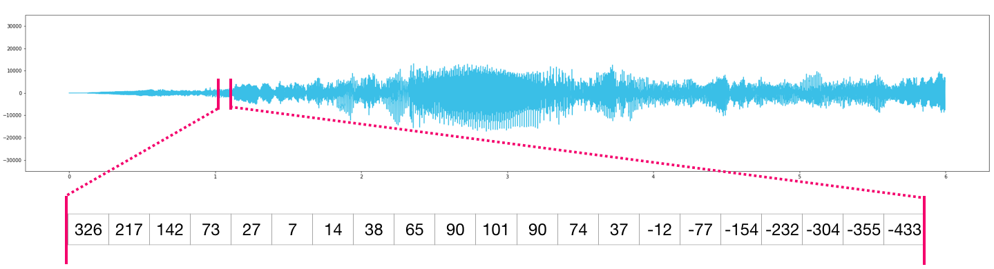
An audio recording is an example of data that can be represented as a 1-dimensional (1-D) array. A 1-D array is also sometimes called a “vector”.

Here the data values in the array are the amplitude values sampled at regular time intervals, and the first (and only) dimension of the array corresponds to the time at which each audio sample should be played.

2-D array (matrix)#

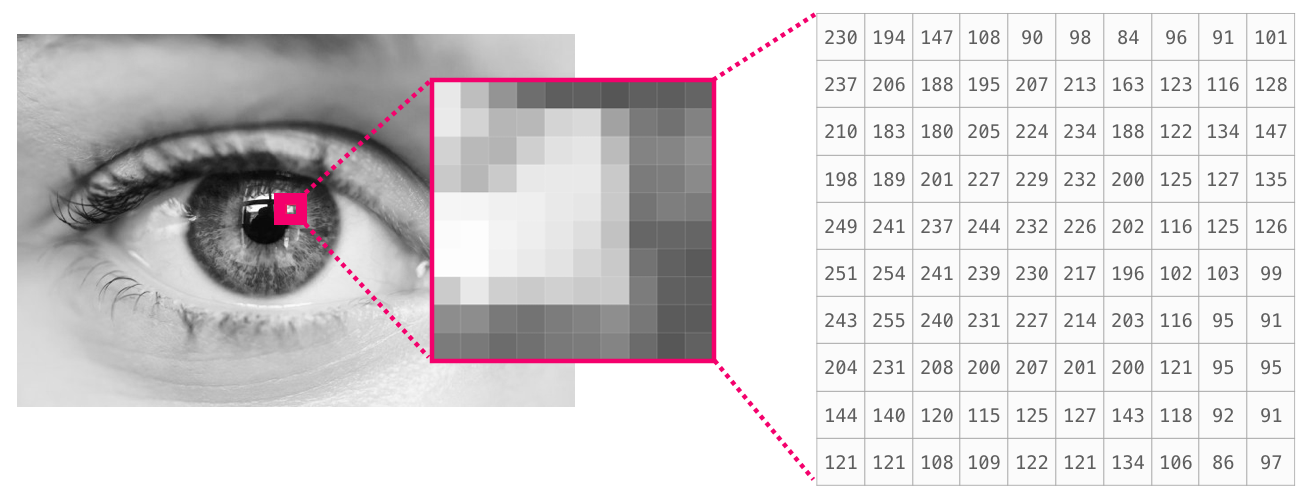
A black-and-white image is an example of data that can be represented as a 2-dimensional (2-D) array. A 2-D array is also sometimes called a “matrix”.

Here the data values in the array correspond to the colour of a pixel, where 0 represents black, 255 represents white, and numbers in between correspond to shades of grey.

The first dimension of the array corresponds to the vertical position of pixels within the image, and the second dimension corresponds to the horizontal position of the pixels.

3-D array (tensor)#

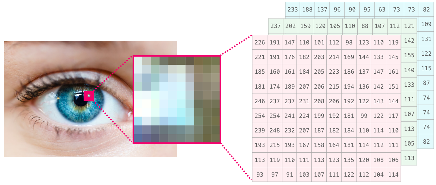
A colour image is an example of data that can be represented as a 3-dimensional (3-D) array. A 3-D array is sometimes also called a “tensor”.

Here the data values represent the intensity of each pixel in three separate colour channels - red, green and blue.

As with the black-and-white image, the first dimension of the array corresponds to the vertical position of pixels within the image, and the second dimension corresponds to the horizontal position of the pixels. Here now there is also a third dimension of length three, which represents the three colour channels.

Genotype calls are another example of data that can be stored as a 3-D array.

Here each data value is an allele encoded numerically, where 0 encodes the reference allele, and higher values encode alternate alleles.

The first dimension (rows) corresponds to the positions in the reference genome; the second dimension (columns) corresponds to the individual organisms that were sequenced; and the third dimension corresponds to the ploidy of the organisms (2 for animals such as humans or mosquitoes).

Importing NumPy#

On colab, NumPy is already installed, so we can go ahead and import it.

import numpy as np

Creating an array from existing data#

There are various ways to create a NumPy array. One way is to create an array from some existing data, via the np.array() function.

Creating a 1-D array#

Let’s create a 1-D array storing the data values [1, 2, 3]. We’ll assign this array to a variable named data, but this variable could be named whatever you like.

data = np.array([1, 2, 3])
data

array([1, 2, 3])

type(data)

numpy.ndarray

Here is a visual illustration of the array we just created.

Every NumPy array has some useful attributes which tell us something about the array.

Here is the number of dimensions:

data.ndim

Here is the total number of elements in the array:

data.size

Here is the shape of the array, which tells us the lengths of each of the dimensions. This returns a tuple of numbers, one length for each dimension. Here there is only one dimension, so we get a tuple of length one.

data.shape

(3,)

Every array also has a data type (dtype) which defines the type of all of the data values.

data.dtype

dtype('int64')

Here “int” means integer, i.e., data values in this array should be interpreted as whole numbers.

Creating a 2-D array#

Let’s create a 2-D array with three rows and two columns.

data_2d = np.array([[1, 2], [3, 4], [5, 6]])
data_2d

array([[1, 2],
       [3, 4],
       [5, 6]])

Here is a visual illustration of this 2-D array.

Again, let’s access the attributes of this array to find out more about it.

data_2d.ndim

data_2d.size

data_2d.shape

(3, 2)

data_2d.dtype

dtype('int64')

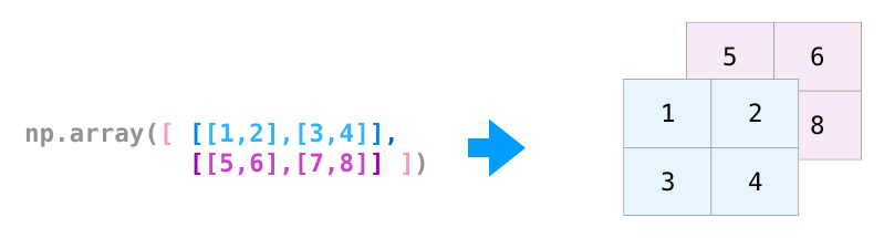
Creating a 3-D array#

Let’s now create a 3-D array, with shape (2, 2, 2) - i.e., all dimensions are length 2.

data_3d = np.array([[[1, 2], [3, 4]], 
                    [[5, 6], [7, 8]]])
data_3d

array([[[1, 2],
        [3, 4]],

       [[5, 6],
        [7, 8]]])

Some other array creation functions#

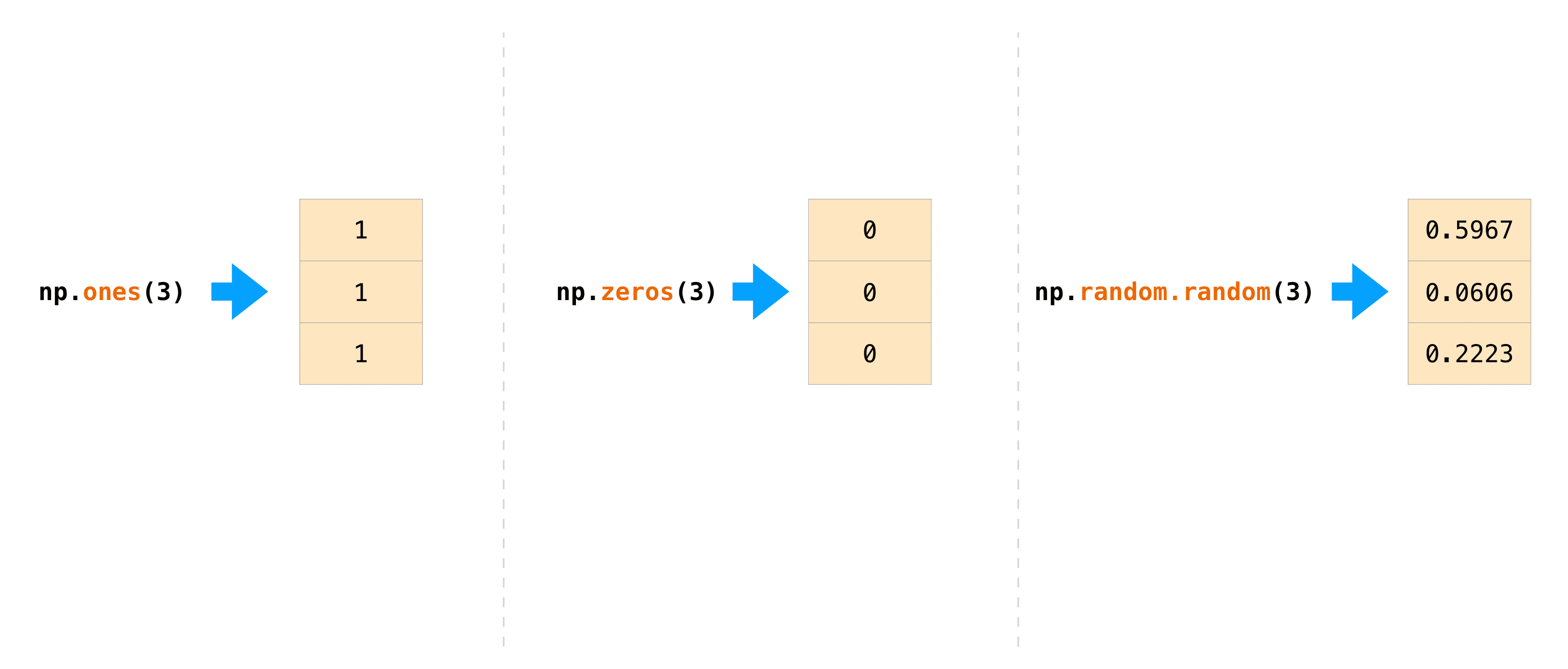
Often it is useful to create an array and initialise it such that all data values are set for us by NumPy. There are several functions for doing this, including np.ones(), np.zeros() and np.random.random().

1-D arrays#

Create an array with all data values initialised to one.

ones = np.ones(3)
ones

array([1., 1., 1.])

ones.ndim

ones.size

ones.shape

(3,)

ones.dtype

dtype('float64')

Note here the dtype is “float64”. Here “float” means floating-point number, i.e., the data values should be interpreted as real numbers (i.e., continuous quantities) with some degree of precision.

Similarly, create an array with all data values initialised to zero.

zeros = np.zeros(3)
zeros

array([0., 0., 0.])

Create an array with data values initialised using a random number generator.

foo = np.random.random(3)
foo

array([0.5086869 , 0.95907072, 0.47661539])

Here are visual illustrations of the three arrays we just created.

Exercise 1 (English)

Uncomment and run the code cells below to answer the following questions.

What is the number of dimensions of the foo array we created above?

What is the number of items (size) of the foo array?

What is the shape of the foo array?

What is the data type of the foo array?

Create an array of ten zeros.

Create an array of one million random numbers.

Exercice 1 (Français)

Décommenter et exécuter les cellules de code ci-dessous pour répondre aux questions suivantes.

Combien de dimensions a l’array foo que nous avons créé plus haut?

Combien d’objets (taille) l’array foo contient-il?

Quel est le type des données de l’array foo?

Créer un array contenant dix zéros.

Créer un array contenant un million de nombres aléatoires.

# foo.ndim

# foo.size

# foo.shape

# foo.dtype

# bar = np.zeros(10)
# bar

# baz = np.random.random(1_000_000)
# baz

2-D arrays#

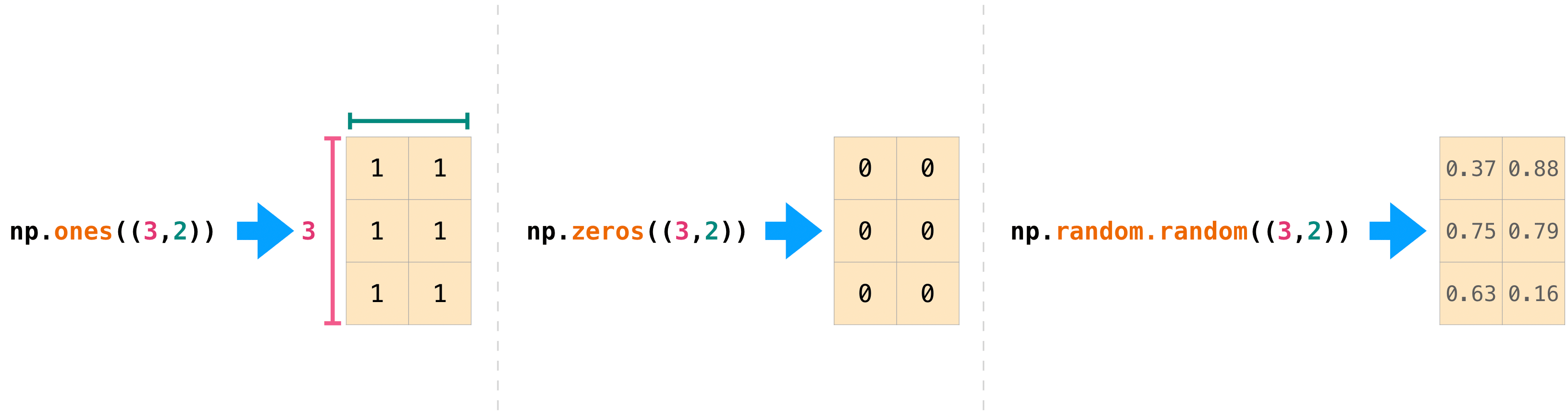
We can also created 2-D arrays via the same functions, by passing the shape of the desired array as the first parameter.

E.g., create an array with three rows and two columns with all data values initialised to one.

ones_2d = np.ones((3, 2))
ones_2d

array([[1., 1.],
       [1., 1.],
       [1., 1.]])

E.g., create an array with three rows and two columns with all data values initialised to zero.

zeros_2d = np.zeros((3, 2))
zeros_2d

array([[0., 0.],
       [0., 0.],
       [0., 0.]])

E.g., create an array with three rows and two columns, initialised with random numbers.

bar = np.random.random((3, 2))
bar

array([[0.47119403, 0.8921313 ],
       [0.10854286, 0.09476291],
       [0.03687078, 0.89322304]])

Here’s an illustration of the 2-D arrays we created.

Exercise 2 (English)

Create a 2-D array of random numbers with 1,000 rows and 500 columns. Check the values of the ndim, size, shape and dtype attributes.

Exercice 2 (Français)

Créer un array de dimension 2 contenant 1000 lignes et 500 colonnes de nombres aléatoires. Vérifier les valeurs des attributs ndim, size, shape et dtype.

Accessing elements of an array (indexing and slicing)#

The data values of an array can be accessed by using the square bracket notation. Remember that indices start from zero in Python.

1-D arrays#

data = np.array([1, 2, 3])
data

array([1, 2, 3])

For 1-D arrays, we write a single index in the square brackets.

E.g., access the data value in the first element of the array:

data[0]

Access the second element:

data[1]

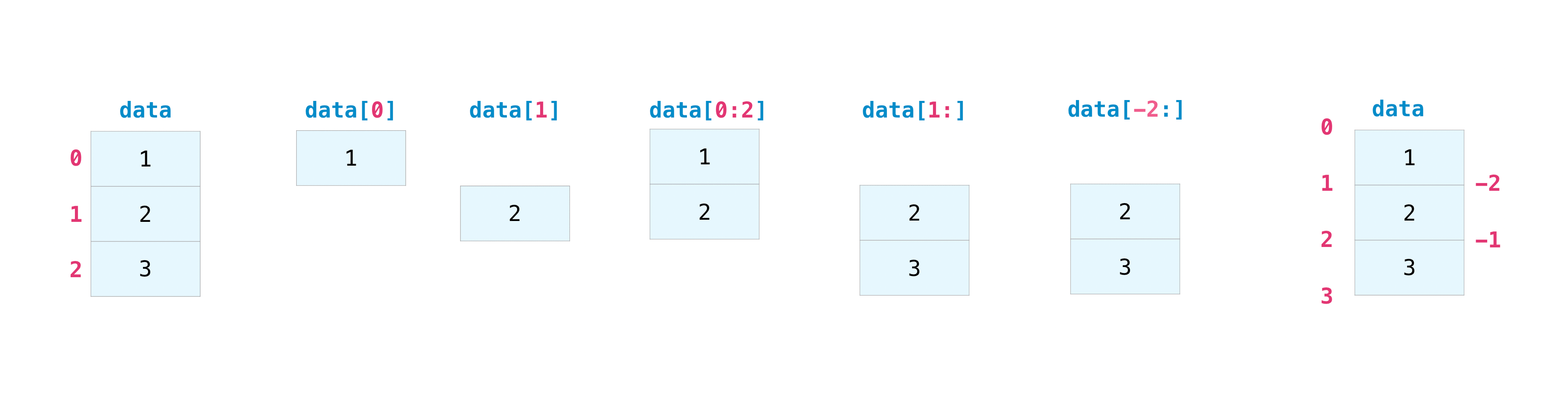
We can also access a contiguous region of an array using the slicing notation, by writing the start and stop indices separated by a colon. Note that this will return a new array. Remember that the start index is included, but the stop index is not.

E.g., access the first two elements:

data[0:2]

array([1, 2])

Access the second and all subsequent elements:

data[1:]

array([2, 3])

Negative indices can also be used, and count backwards from the end of an array.

E.g., access the second from last and all subsequent elements:

data[-2:]

array([2, 3])

Here is an illustration of the array we created, and the results of indexing the array in different ways.

Exercise 3 (English)

Create a new 1-D array initialised with the data values [0, 5, 23, 37, 42, 54, 61, 79, 88, 90].

Using indexing to access the data value in the fifth element of the array.

Access the final element of the array.

Using slicing to access the third, fourth and fifth elements of the array.

Exercice 3 (Français)

Créer un array de dimension 1 contenant les valeurs [0, 5, 23, 37, 42, 54, 61, 79, 88, 90].

Utiliser un index pour accéder à la valeur du cinquième élément de cet array.

Accéder au dernier élément de cet array.

Utiliser une tranche pour accéder au troisième, quatrième et cinquième éléments de cet array.

2-D arrays#

2-D arrays can also be indexed using the square bracket notation. Here, because there are two dimensions, we need to provide two indices, one for each dimension.

data = np.array([[1, 2], [3, 4], [5, 6]])
data

array([[1, 2],
       [3, 4],
       [5, 6]])

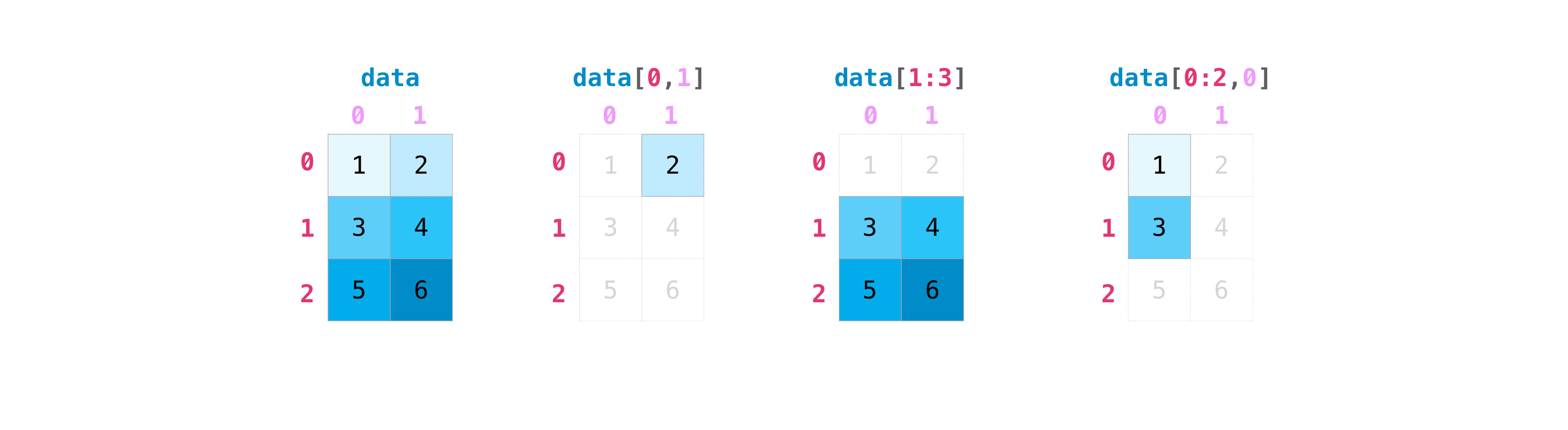
E.g., access the data value in the first row, second column:

data[0, 1]

We can also slice 2-D arrays.

E.g., access the second and all subsequent rows, and all columns:

data[1:3]

array([[3, 4],
       [5, 6]])

To be more explicit, we could also provide the slice we require along the second dimension, i.e., all columns:

data[1:3, :]

array([[3, 4],
       [5, 6]])

Access the first two rows, first column:

data[0:2, 0]

array([1, 3])

Here’s an illustration of these indexing operations on a 2-D array:

Exercise 4 (English)

Create a new 2-D array initialised with the data values [[0, 5, 23], [37, 42, 54], [61, 79, 88]].

Use indexing to access the data value in second row, third column of the array.

Use slicing to access the first and second rows of the array.

Access the last two values in the second column of the array.

Exercice 4 (Français)

Créer un nouvel array de dimension 2 contenant les valeurs [[0, 5, 23], [37, 42, 54], [61, 79, 88]].

Utiliser les indexes pour accéder à la valeur se trouvant à la deuxième ligne, troisième colonne de cet array.

Utiliser une tranche pour accéder à la première et à la seconde ligne de cet array.

Accéder aux deux dernières valeurs de la seconde colonne de cet array.

Basic mathematical operations with arrays#

One of the most powerful features of NumPy arrays is that you can use them to perform mathematical operations. In particular, you can apply mathematical operations between entire arrays, without having to write any for loops. Let’s see this in action.

1-D arrays#

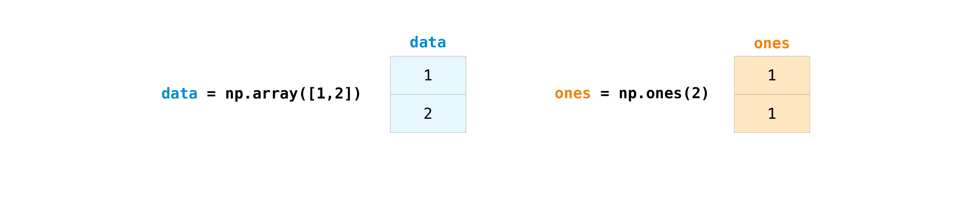
To demonstrate, let’s create two arrays.

data = np.array([1, 2])
ones = np.ones(2)

Now, add these two arrays together.

result = data + ones
result

array([2., 3.])

Each element of the data array has been added to each element of the ones array, to create a new array that we’ve assigned to the variable named result. This is an example of an elementwise computation that NumPy performs for us.

Here’s an illustration of this computation:

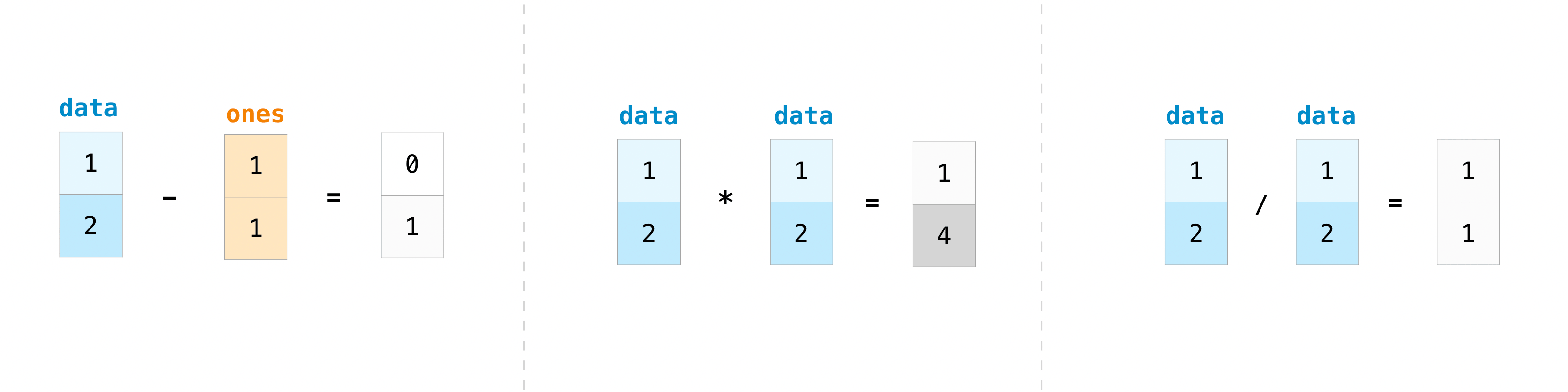
Similarly, we can subtract, multiply and divide arrays.

data - ones

array([0., 1.])

data * data

array([1, 4])

data / data

array([1., 1.])

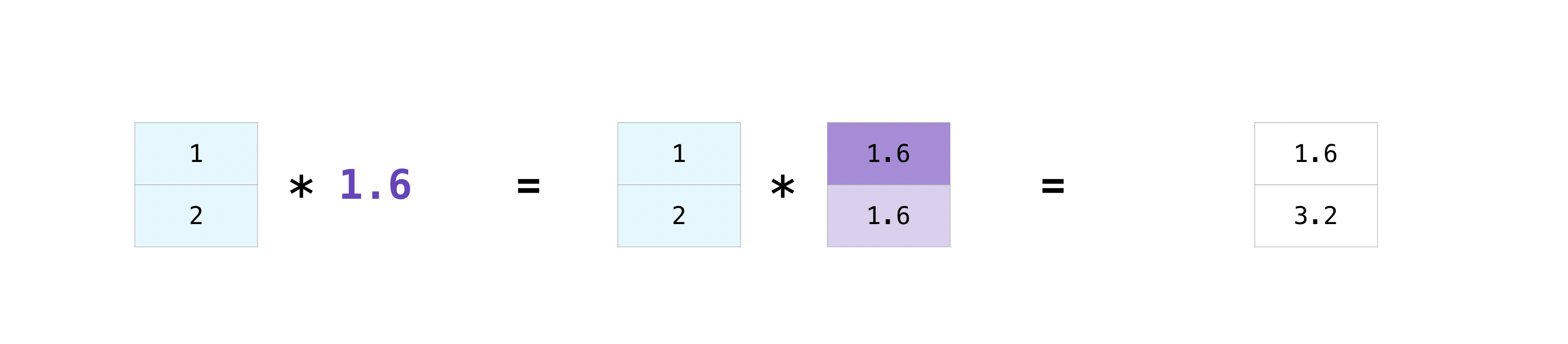
You can also perform arithmetic between arrays and a single number (also known as a scalar). E.g., multiply all values in the data array by the number 1.6:

data * 1.6

array([1.6, 3.2])

Here, NumPy has guessed that we want to multiply each element of the data array. Do it has “broadcast” the scalar value 1.6 to an array of the same shape as data. This is an illustration of what happened:

As well as arithmetic, you can also perform comparisons. E.g., compute all values in the data array that are greater than one:

result = data > 1
result

array([False,  True])

Note that the result is an array of Boolean values (either True or False).

result.dtype

dtype('bool')

2-D arrays#

All of the same mathematical operations can be performed with 2-D arrays as well.

E.g., add two arrays:

data = np.array([[1, 2], [3, 4]])
ones = np.ones((2, 2))
data + ones

array([[2., 3.],
       [4., 5.]])

E.g., multiply an array by a scalar:

data * 1.6

array([[1.6, 3.2],
       [4.8, 6.4]])

E.g., compare an array with a scalar:

data > 1

array([[False,  True],
       [ True,  True]])

Exercise 5 (English)

Create a new array initialised with the data values [[0, 5, 23], [37, 42, 54], [61, 79, 88]].

Multiply this array by itself.

Add one to every element of this array.

Exercice 5 (Français)

Créer un nouvel array initialisé avec les valeurs [[0, 5, 23], [37, 42, 54], [61, 79, 88]].

Multiplier cet array par lui-même.

Ajouter un à chaque élément de cet array.

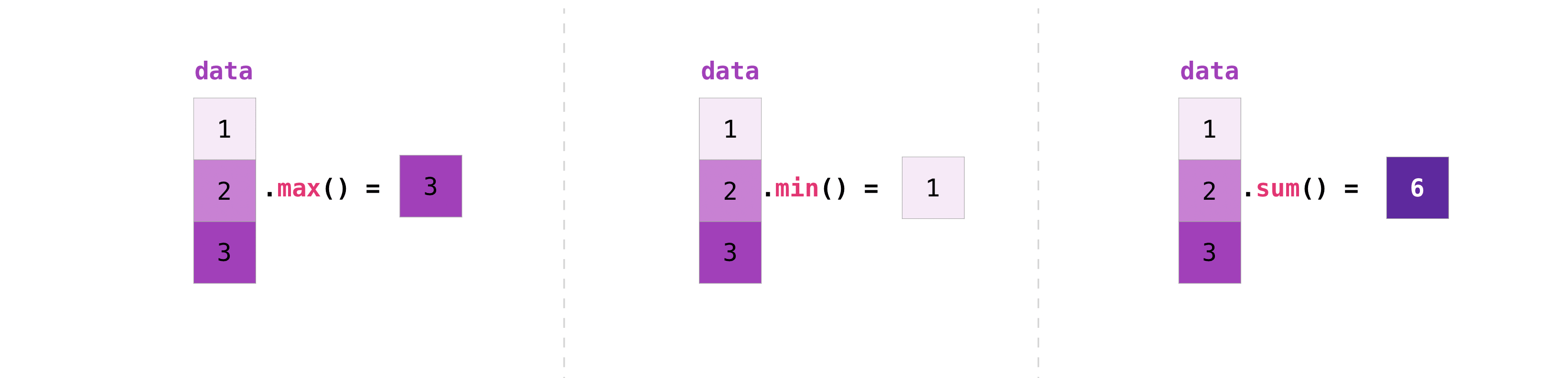
Aggregations#

NumPy also provides some aggregation functions, including max(), min(), sum(), and count_nonzero(), which you can use with arrays.

Note that max(), min() and sum() can be called in two different ways: either as methods of an array, or as a function.

1-D arrays#

Here are examples of aggregation functions used with a 1-D array.

data = np.array([1, 2, 3])

data.max()

np.max(data)

data.min()

data.sum()

data > 1

array([False,  True,  True])

np.count_nonzero(data > 1)

2-D arrays#

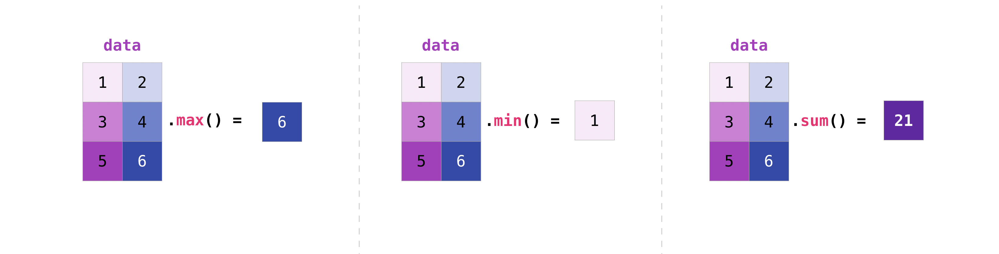
Here are examples of aggregation functions used with a 2-D array.

data = np.array([[1, 2], [3, 4], [5, 6]])
data

array([[1, 2],
       [3, 4],
       [5, 6]])

data.max()

data.min()

data.sum()

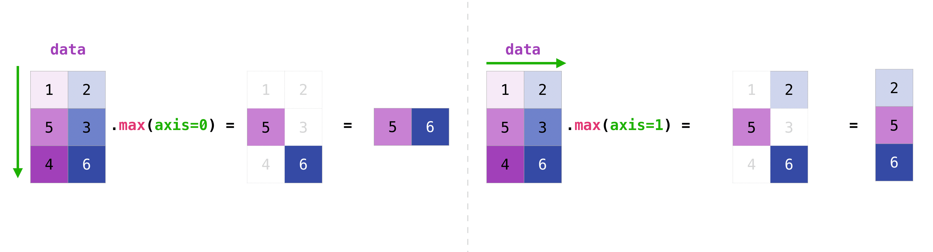
The axis parameter can also be used here to perform aggregation along a dimension of an array.

data.max(axis=0)

array([5, 6])

data.max(axis=1)

array([2, 4, 6])

data > 1

array([[False,  True],
       [ True,  True],
       [ True,  True]])

np.count_nonzero(data > 1)

np.count_nonzero(data > 1, axis=1)

array([1, 2, 2])

Exercise 6 (English)

Create a 2-D array of random numbers with 4 rows and 3 columns.

Multiply the array by 100.

Find the maximum, minimum and sum of the array.

Find the maximum value in each row.

Find the minimum value in each column.

Exercice 6 (Français)

Créer un array de dimension 2 avec 4 lignes et 3 colonnes de nombres aléatoires.

Multiplier cet array par 100.

Trouver le maximum, le minimum et la somme de cet array.

Trouver le maximum de chaque ligne.

Trouver le minimum de chaque colonne.

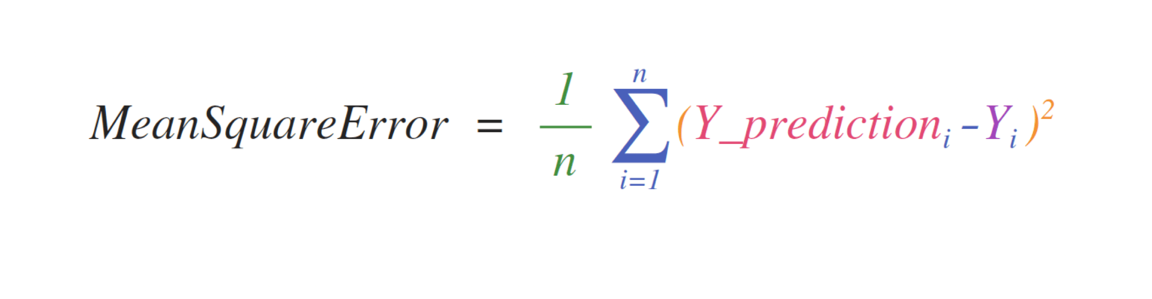
Working with mathematical formulas#

NumPy can be used to implement mathematical formulas and perform some computation over data of any size.

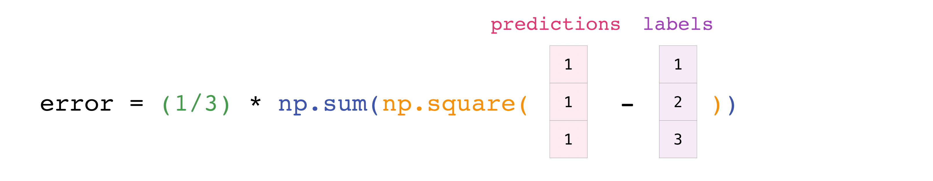
For example, here is a formula for computing mean square error.

To illustrate how we would implement this with NumPy, let’s create some data:

predictions = np.array([1, 1, 1])
predictions

array([1, 1, 1])

labels = np.array([1, 2, 3])
labels

array([1, 2, 3])

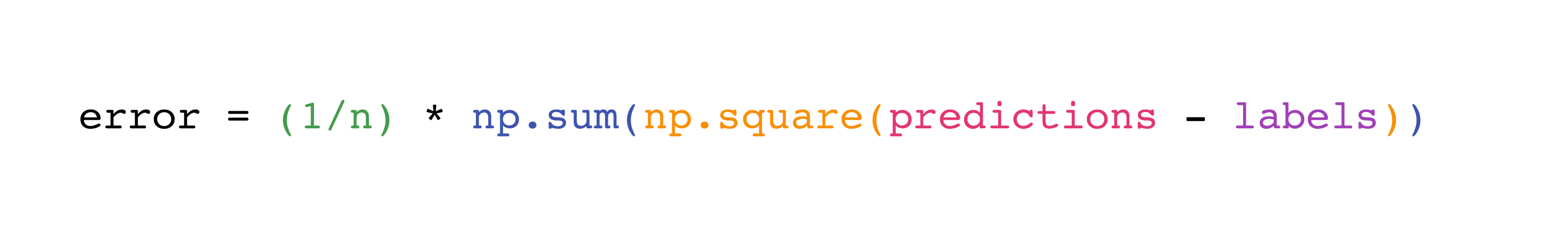
Now implement the formula to compute the mean square error between predictions and labels:

n = predictions.size
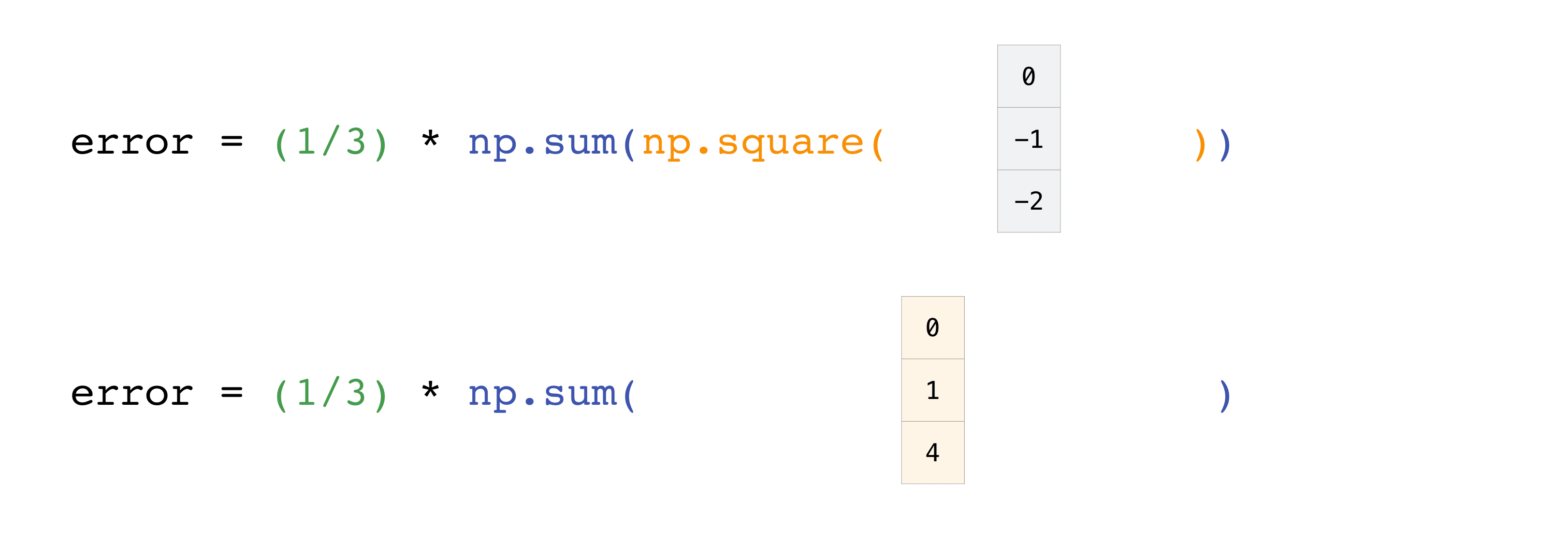
error = (1/n) * np.sum(np.square(predictions - labels))
error

1.6666666666666665

Here is a visual illustration of how NumPy performs this computation internally.

In fact, there is an even simpler way we could compute this, using the np.mean() function:

error = np.mean(np.square(predictions - labels))
error

1.6666666666666667

Of course, the best part about this is, it doesn’t matter how much data we have - we could pass arrays of any size into this computation.

Data types (dtypes)#

Finally, let’s take a very brief look at some of the different data types that NumPy supports.

At the beginning of this module, we created an array from some existing data values using np.array().

data = np.array([1, 2, 3])
data

array([1, 2, 3])

Because of the data values we provided, NumPy chose an integer data type for us:

data.dtype

dtype('int64')

Earlier, we created an array of zeros using the np.zeros() function.

zeros = np.zeros(3)
zeros

array([0., 0., 0.])

By default, NumPy created this array with a floating-point data type:

zeros.dtype

dtype('float64')

If we knew we only wanted to store whole numbers, we could have used the dtype parameter to override the default, e.g.:

zeros = np.zeros(3, dtype=np.int64)
zeros

array([0, 0, 0])

zeros.dtype

dtype('int64')

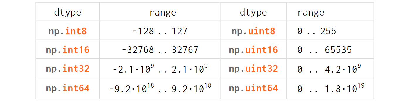
Here are all of the integer data types that NumPy supports, along with the range of possible data values for each:

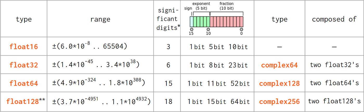
Here are all of the floating-point data types that NumPy currently supports, along with the range of possible data values for each:

Module 1 - NumPy arrays

Contents

Module 1 - NumPy arrays#

Learning objectives#

Lecture#

English#

Français#

Why use NumPy?#

What is a NumPy array?#

1-D array (vector)#

2-D array (matrix)#

3-D array (tensor)#

Importing NumPy#

Creating an array from existing data#

Creating a 1-D array#

Creating a 2-D array#

Creating a 3-D array#

Some other array creation functions#

1-D arrays#

2-D arrays#

Accessing elements of an array (indexing and slicing)#

1-D arrays#

2-D arrays#

Basic mathematical operations with arrays#

1-D arrays#

2-D arrays#

Aggregations#

1-D arrays#

2-D arrays#

Working with mathematical formulas#

Data types (dtypes)#

Further reading#