Module 1 - Organophosphate resistance markers (combining SNP and CNV data)

Module 1 - Organophosphate resistance markers (combining SNP and CNV data)#

Theme: Analysis

The acetylcholinesterase enzyme produced by the Ace1 gene is the target for organophosphate insecticides. Both target-site mutations and gene copy number amplifications have been implicated in insecticide resistance phenotypes.

Overexpression of the Gste2 gene has also been associated with resistance to some organophosphates, and SNPs in the same gene have been linked to pyrethroid and DDT resistance phenotypes.

In this module we’re going to investigate known organophosphate insecticide resistance markers, learning how to combine SNPs and CNVs, using data from Ag3.0.

Learning Objectives#

Understand mechanisms and markers of organophosphate resistance.
Revisit amino acid frequency and CNV gene frequency analyses.
Learn how to combine and interpret SNP and CNV frequency data.

Lecture#

English#

Français#

Please note that the code in the cells below might differ from that shown in the video. This can happen because Python packages and their dependencies change due to updates, necessitating tweaks to the code.

Setup#

First, let’s begin by installing and importing some Python packages, and configuring access to Anopheles genomic data from the MalariaGEN Ag3.0 data resource.

%pip install -q --no-warn-conflicts malariagen_data

Note: you may need to restart the kernel to use updated packages.

import malariagen_data

import warnings
warnings.simplefilter(action='ignore', category=Warning)

import pandas as pd

Note that authentication is required to access data through the package, please follow the instructions here.

ag3 = malariagen_data.Ag3()
ag3

MalariaGEN Ag3 API client
Please note that data are subject to terms of use, for more information see the MalariaGEN website or contact support@malariagen.net. See also the Ag3 API docs.
Storage URL	gs://vo_agam_release/
Data releases available	3.0, 3.1, 3.2, 3.3, 3.4, 3.5, 3.6, 3.7, 3.8, 3.9
Results cache	None
Cohorts analysis	20240418
AIM analysis	20220528
Site filters analysis	dt_20200416
Software version	malariagen_data 9.0.0
Client location	unknown

Introduction#

The Ace1 gene#

Acetylcholinesterase, also known as AChE, is an essential carboxylesterase enzyme in the nervous system of animals. AChE breaks down the neurotransmitter acetylcholine.

In anophelines, the AChE protein is produced by the Ace1 gene.

In the diagram below we see the neurotransmitter acetylcholine (ACh) being released from the pre-synaptic membrane of one neuron in the nervous system, and binding to receptors on the post-synaptic membrane of another neuron. This enables a nerve impulse to travel between the neurons. AChE (the red “Pac Man”) breaks ACh down into acetate and choline, terminating the nerve impulse.

Figure reference: Muramatsu I, Masuoka T, Uwada J, et al. A New Aspect of Cholinergic Transmission in the Central Nervous System. 2018 Apr 4. In: Akaike A, Shimohama S, Misu Y, editors. Nicotinic Acetylcholine Receptor Signaling in Neuroprotection [Internet]. Singapore: Springer; 2018. http://creativecommons.org/licenses/by/4.0/

Resistance to arganophosphate and carbamate insecticides#

Organophosphate (OP) and carbamate insecticides block the action of AChE via competitive binding. This results in nerve impulses not being terminated, and leads to insect death.

Non-synonymous “target-site” mutations in Ace1 can confer resistance to both carbamate and OP insecticides by reducing how well they bind to AChE. However, these mutations make AChE less effective in the absence of insecticides. Due to the important role that AChE plays in the nervous system, these resistant phenotypes come with a high fitness cost.

Amplifications of the Ace1 gene have also been found to be associated with carbamate and OP resistance. It is thought that these amplifications, detectable using CNV analyses, may increase resistance phenotype by enabling more copies of the mutant gene to be present while restoring mosquito fitness in the absence of insecticides by allowing a un-mutated (wild-type) copy of the gene to remain.

Pirimiphos methyl (PM) is an OP insecticide used for indoor residual spraying (IRS). With the increase of pyrethroid and carbamate resistance, WHO has recommend PM for IRS since 2013. PM is the active ingredient in the IRS product Actellic CS, and is now being widely used, hence the importance of tracking known OP resistance markers.

Ace1 amino acid substitution frequencies#

Xavier Grau-Bové and colleagues demonstrated that, in Anopheles gambiae and colluzii from West Africa, the G280S amino acid altering SNP in the Ace1 gene was associated with resistance to the OP pirimiphos methyl (Grau-Bové et al. 2021).

Let’s examine Ace1 amino acid allele frequencies in An. coluzzi (West & Central Africa) from the Ag3.0 data release using the ag3.aa_allele_frequencies() function.

In brief, this analysis will take each amino acid in the Ace1 gene in turn, and calculate the frequency of alternative (non-reference) residues in each of our chosen mosquito cohorts.

For example, if we take the figure below and consider the locus of interest to be an amino acid in the Ace1 gene, we see that from our cohort of five individuals (ten haplotypes), there are four instances of an alternative amino acid. This means the allele frequency of the alternative amino acid here is 0.4.

A deep dive into the aa_allele_frequencies() function and allele frequencies in general can be found in workshop 1 - module 4, where we used it to investigate SNP and amino acid substitution frequencies in the Vgsc gene (the target of pyrethroid and DDT insecticides).

Using ? we can remind ourselves what parameters we need for this function.

ag3.aa_allele_frequencies?

ace1_aa_freqs_df = ag3.aa_allele_frequencies(
    transcript="AGAP001356-RA", 
    sample_sets = '3.0',
    cohorts="admin1_year",
    sample_query='taxon == "coluzzii"'
)

ace1_aa_freqs_df

			frq_AO-LUA_colu_2009	frq_BF-09_colu_2012	frq_BF-09_colu_2014	frq_CF-BGF_colu_1994	frq_CI-LG_colu_2012	frq_CM-CE_colu_2013	frq_GH-AA_colu_2012	frq_GH-CP_colu_2012	frq_GH-WP_colu_2012	frq_GM-L_colu_2006	...	transcript	aa_pos	ref_allele	ref_aa	alt_aa	effect	impact	alt_allele	max_af	label
aa_change	contig	position
R4G	2R	3489222	0.000000	0.006098	0.000000	0.0	0.0000	0.0	0.000000	0.00	0.0	0.0	...	AGAP001356-RA	4.0	C	R	G	NON_SYNONYMOUS_CODING	MODERATE	G	0.006098	R4G (2R:3,489,222 C>G)
P19T	2R	3489267	0.000000	0.000000	0.000000	0.0	0.0000	0.0	0.000000	0.00	0.0	0.0	...	AGAP001356-RA	19.0	C	P	T	NON_SYNONYMOUS_CODING	MODERATE	A	0.018519	P19T (2R:3,489,267 C>A)
G24C	2R	3489282	0.006173	0.000000	0.000000	0.0	0.0000	0.0	0.000000	0.00	0.0	0.0	...	AGAP001356-RA	24.0	G	G	C	NON_SYNONYMOUS_CODING	MODERATE	T	0.006173	G24C (2R:3,489,282 G>T)
G24S	2R	3489282	0.000000	0.000000	0.000000	0.0	0.0000	0.0	0.000000	0.00	0.0	0.0	...	AGAP001356-RA	24.0	G	G	S	NON_SYNONYMOUS_CODING	MODERATE	A	0.018519	G24S (2R:3,489,282 G>A)
V25L	2R	3489285	0.000000	0.000000	0.000000	0.0	0.0000	0.0	0.000000	0.00	0.0	0.0	...	AGAP001356-RA	25.0	G	V	L	NON_SYNONYMOUS_CODING	MODERATE	T	0.020000	V25L (2R:3,489,285 G>T)
...	...	...	...	...	...	...	...	...	...	...	...	...	...	...	...	...	...	...	...	...	...	...	...
V726M	2R	3493750	0.000000	0.000000	0.009434	0.0	0.0000	0.0	0.000000	0.00	0.0	0.0	...	AGAP001356-RA	726.0	G	V	M	NON_SYNONYMOUS_CODING	MODERATE	A	0.009434	V726M (2R:3,493,750 G>A)
A731T	2R	3493765	0.000000	0.000000	0.000000	0.0	0.0000	0.0	0.000000	0.00	0.0	0.0	...	AGAP001356-RA	731.0	G	A	T	NON_SYNONYMOUS_CODING	MODERATE	A	0.002907	A731T (2R:3,493,765 G>A)
A731V	2R	3493766	0.000000	0.012195	0.009434	0.0	0.0125	0.0	0.000000	0.00	0.0	0.0	...	AGAP001356-RA	731.0	C	A	V	NON_SYNONYMOUS_CODING	MODERATE	T	0.012500	A731V (2R:3,493,766 C>T)
V733A	2R	3493772	0.000000	0.006098	0.000000	0.0	0.0000	0.0	0.035714	0.00	0.0	0.0	...	AGAP001356-RA	733.0	T	V	A	NON_SYNONYMOUS_CODING	MODERATE	C	0.035714	V733A (2R:3,493,772 T>C)
R734T	2R	3493775	0.000000	0.000000	0.000000	0.0	0.0000	0.0	0.000000	0.02	0.0	0.0	...	AGAP001356-RA	734.0	G	R	T	NON_SYNONYMOUS_CODING	MODERATE	C	0.020000	R734T (2R:3,493,775 G>C)

159 rows × 26 columns

We get 159 amino acid changes from our coluzzii cohorts, but many are at low frequencies. Let’s filter our DataFrame using query to just alternative amino acid frequencies greater than, or equal to 5%.

ace1_aa_filt_df = ace1_aa_freqs_df.query("max_af >= 0.05")
ace1_aa_filt_df

			frq_AO-LUA_colu_2009	frq_BF-09_colu_2012	frq_BF-09_colu_2014	frq_CF-BGF_colu_1994	frq_CI-LG_colu_2012	frq_CM-CE_colu_2013	frq_GH-AA_colu_2012	frq_GH-CP_colu_2012	frq_GH-WP_colu_2012	frq_GM-L_colu_2006	...	transcript	aa_pos	ref_allele	ref_aa	alt_aa	effect	impact	alt_allele	max_af	label
aa_change	contig	position
F35S	2R	3489316	1.000000	0.975610	1.000000	1.000000	0.99375	1.000000	1.000000	1.00	1.000000	0.973684	...	AGAP001356-RA	35.0	T	F	S	NON_SYNONYMOUS_CODING	MODERATE	C	1.000000	F35S (2R:3,489,316 T>C)
G61D	2R	3489394	0.061728	0.000000	0.000000	0.000000	0.00000	0.041667	0.000000	0.00	0.000000	0.000000	...	AGAP001356-RA	61.0	G	G	D	NON_SYNONYMOUS_CODING	MODERATE	A	0.061728	G61D (2R:3,489,394 G>A)
A65S	2R	3489405	1.000000	0.597561	0.660377	0.923077	0.70000	0.791667	0.678571	0.66	0.729167	0.315789	...	AGAP001356-RA	65.0	G	A	S	NON_SYNONYMOUS_CODING	MODERATE	T	1.000000	A65S (2R:3,489,405 G>T)
R106H	2R	3489529	0.000000	0.000000	0.000000	0.000000	0.00000	0.208333	0.000000	0.00	0.000000	0.000000	...	AGAP001356-RA	106.0	G	R	H	NON_SYNONYMOUS_CODING	MODERATE	A	0.208333	R106H (2R:3,489,529 G>A)
V218L	2R	3491888	0.000000	0.018293	0.028302	0.000000	0.00000	0.000000	0.035714	0.02	0.000000	0.000000	...	AGAP001356-RA	218.0	G	V	L	NON_SYNONYMOUS_CODING	MODERATE	T	0.060000	V218L (2R:3,491,888 G>T)
G280S	2R	3492074	0.000000	0.024390	0.018868	0.000000	0.43750	0.000000	0.285714	0.00	0.000000	0.000000	...	AGAP001356-RA	280.0	G	G	S	NON_SYNONYMOUS_CODING	MODERATE	A	0.437500	G280S (2R:3,492,074 G>A)
S338R	2R	3492329	0.000000	0.024390	0.000000	0.000000	0.00000	0.000000	0.000000	0.00	0.020833	0.000000	...	AGAP001356-RA	338.0	C	S	R	NON_SYNONYMOUS_CODING	MODERATE	A	0.055556	S338R (2R:3,492,329 C>A)
S367A	2R	3492414	0.000000	0.000000	0.000000	0.000000	0.00000	0.000000	0.000000	0.00	0.000000	0.000000	...	AGAP001356-RA	367.0	T	S	A	NON_SYNONYMOUS_CODING	MODERATE	G	0.050000	S367A (2R:3,492,414 T>G)
D624E	2R	3493273	0.000000	0.000000	0.000000	0.115385	0.01250	0.000000	0.035714	0.00	0.020833	0.000000	...	AGAP001356-RA	624.0	C	D	E	NON_SYNONYMOUS_CODING	MODERATE	A	0.115385	D624E (2R:3,493,273 C>A)
N645I	2R	3493401	0.000000	0.006098	0.009434	0.000000	0.01250	0.000000	0.035714	0.00	0.000000	0.000000	...	AGAP001356-RA	645.0	A	N	I	NON_SYNONYMOUS_CODING	MODERATE	T	0.090909	N645I (2R:3,493,401 A>T)
S648N	2R	3493410	0.000000	0.012195	0.009434	0.000000	0.00000	0.208333	0.000000	0.00	0.000000	0.000000	...	AGAP001356-RA	648.0	G	S	N	NON_SYNONYMOUS_CODING	MODERATE	A	0.208333	S648N (2R:3,493,410 G>A)

11 rows × 26 columns

Now we have just 11 amino acid substitutions of interest, including the G280S mutation implicated in organophosphate insecticide resistance.

Let’s display the pandas DataFrame as a heatmap for ease of visualisation.

ag3.plot_frequencies_heatmap(ace1_aa_filt_df, height=600, width=1000)

There are few high frequency amino acid substitutions in Ace1, as we might expect for a functionally constrained gene. However, we can see appreciable frequencies of the known organophosphate resistance marker G280S in cohorts from Cote d’Ivoire (CI-LG_colu_2012) and Ghana (GH-AA_colu_2012). There are also high frequencies of F35S and A65S mutations across all the cohorts. In the case of F35S, this may well be an artifact, driven by the mutant allele actually being in the reference genome so the wild-type (S) appears as the high frequency alternative allele. The A65F mutation is present in all populations at varying frequencies, but we can see that it is found at high frequency in the Central African Republic cohort collected in 1994, prior to OP use in malaria control.

Ace1 copy number variation frequencies#

Increases in copy number of the Ace1 gene have been linked with insecticide resistance in association with the G280S amino acid subsitution in both Anopheles and Culex mosquitoes.

In Culex, the 280S mutation has been shown to cause over 60% reduction in esterase enzymatic activity in the absence of insecticide, causing developmental and behavioural issues. It is likely that the same mutation causes similar issues in Anopheles.

As we can see in the figure below, a permanent “heterozygote” can be created by pairing a wild type 280G carrying Ace1 gene with at least one OP resistance mutation 280S carrying Ace1 gene, on the same haplotype.

This haplotypic heterozygote compensates for the neurophysiological fitness cost of 280S in the absence of insecticide. Plus there can be a number of copies of the resistant gene and carrying multiple copies has been strongly associated with increased carbamate resistance in bioassays (Edi et al. 2012).

Let’s use the CNV data to look into copy number of the the Ace1 gene in An. coluzzii from the Ag3.0 data set. We can use the ag3.plot_cnv_hmm_heatmap() function (explored in detail in workshop 2 - module 3 to visualise copy number around Ace1.

Briefly, this function builds a heatmap of genomic copy number per individual mosquito across a region of interest.

ag3.plot_cnv_hmm_heatmap?

ag3.plot_cnv_hmm_heatmap(
    region='2R:3,300,000-4,000,000',
    sample_query='taxon == "coluzzii"',
    sample_sets='AG1000G-CI', 
    row_height=6
);

We can see that many of the coluzzii samples in the Cote d’Ivoire sample set have amplifications in the region of the Ace1 gene, of 3, or 4+ copies.

This fits with what we know from previous research showing that amplifications appear common in Cote d’Ivoire (Grau-Bové et al. 2021).

We can summarise the same data as frequency of amplification/deletion per cohort using the ag3.gene_cnv_frequencies() function that we learned about in workshop 2 - module 4.

Briefly, this function summarises gene amplification and deletion over each cohort of mosquitoes, so that we can estimate the fraction of mosquitoes from a given time, place and species that carry some form of copy number variation at a given gene of interest. It ignores whether the individual was heterozygous or homozygous for that CNV, and also ignores the actual number of additional copies that may be present.

ag3.gene_cnv_frequencies?

ace1_cnv_freqs_df = ag3.gene_cnv_frequencies(
    region="2R:3,483,099-3,497,400",
    sample_sets = '3.0',
    cohorts="admin1_year",
    sample_query='taxon == "coluzzii"'
)
ace1_cnv_freqs_df

			gene_strand	gene_description	contig	start	end	frq_AO-LUA_colu_2009	frq_BF-09_colu_2012	frq_BF-09_colu_2014	frq_CF-BGF_colu_1994	frq_CI-LG_colu_2012	...	frq_GH-WP_colu_2012	frq_GM-M_colu_2012	frq_GN-N_colu_2012	frq_ML-2_colu_2004	frq_ML-2_colu_2014	frq_ML-3_colu_2012	frq_ML-4_colu_2004	max_af	windows	label
gene_id	gene_name	cnv_type
AGAP001356	ACE1	amp	+	Acetylcholinesterase [Source:UniProtKB/Swiss-P...	2R	3483099	3497400	0.0	0.0375	0.037736	0.0	0.87013	...	0.0	0.0	0.0	0.0	0.0	0.038462	0.0	0.87013	48	AGAP001356 (ACE1) amp

1 rows × 22 columns

We only have one row in this DataFrame as there is just one gene (Ace1) within the region parameter we provided and there are only amplification CNVs (“amp”) detected in our cohorts, no deletions. Consequently, we don’t need to apply any filtering here.

Let’s visualise this DataFrame as a heatmap.

ag3.plot_frequencies_heatmap(ace1_cnv_freqs_df, height=300, width=1000)

This gene frequencies summary makes the CNV data much easier to interpret. We can now clearly see that Amplifications of the Ace1 gene appear rare in our coluzzii samples, apart from a cohort from Ghana and the cohort from Cote d’Ivoire.

Combining SNP and CNV allele frequencies#

Given that an association between the G280S substitution, Ace1 gene amplification, and insecticide resistance has been shown, it will be useful to visualise the amino acid (SNP) frequencies and the CNV gene frequencies together.

You may have noticed that the frequency DataFrame output is similar for both ag3.aa_allele_frequencies(() and ag3.gene_cnv_frequencies(), with the cohort frequency columns named with a string starting with “frq”. This makes it easy to combine the outputs from our two analyses and visualise the results together.

First we simply combine the two DataFrames along the rows axis (axis=0) using pandas.concat().

ace1_combined_df = pd.concat(
    [ace1_aa_filt_df, ace1_cnv_freqs_df], 
    axis=0,  # concatenate rows
)

ace1_combined_df

			frq_AO-LUA_colu_2009	frq_BF-09_colu_2012	frq_BF-09_colu_2014	frq_CF-BGF_colu_1994	frq_CI-LG_colu_2012	frq_CM-CE_colu_2013	frq_GH-AA_colu_2012	frq_GH-CP_colu_2012	frq_GH-WP_colu_2012	frq_GM-L_colu_2006	...	impact	alt_allele	max_af	label	gene_strand	gene_description	contig	start	end	windows
F35S	2R	3489316	1.000000	0.975610	1.000000	1.000000	0.99375	1.000000	1.000000	1.00	1.000000	0.973684	...	MODERATE	C	1.000000	F35S (2R:3,489,316 T>C)	NaN	NaN	NaN	NaN	NaN	NaN
G61D	2R	3489394	0.061728	0.000000	0.000000	0.000000	0.00000	0.041667	0.000000	0.00	0.000000	0.000000	...	MODERATE	A	0.061728	G61D (2R:3,489,394 G>A)	NaN	NaN	NaN	NaN	NaN	NaN
A65S	2R	3489405	1.000000	0.597561	0.660377	0.923077	0.70000	0.791667	0.678571	0.66	0.729167	0.315789	...	MODERATE	T	1.000000	A65S (2R:3,489,405 G>T)	NaN	NaN	NaN	NaN	NaN	NaN
R106H	2R	3489529	0.000000	0.000000	0.000000	0.000000	0.00000	0.208333	0.000000	0.00	0.000000	0.000000	...	MODERATE	A	0.208333	R106H (2R:3,489,529 G>A)	NaN	NaN	NaN	NaN	NaN	NaN
V218L	2R	3491888	0.000000	0.018293	0.028302	0.000000	0.00000	0.000000	0.035714	0.02	0.000000	0.000000	...	MODERATE	T	0.060000	V218L (2R:3,491,888 G>T)	NaN	NaN	NaN	NaN	NaN	NaN
G280S	2R	3492074	0.000000	0.024390	0.018868	0.000000	0.43750	0.000000	0.285714	0.00	0.000000	0.000000	...	MODERATE	A	0.437500	G280S (2R:3,492,074 G>A)	NaN	NaN	NaN	NaN	NaN	NaN
S338R	2R	3492329	0.000000	0.024390	0.000000	0.000000	0.00000	0.000000	0.000000	0.00	0.020833	0.000000	...	MODERATE	A	0.055556	S338R (2R:3,492,329 C>A)	NaN	NaN	NaN	NaN	NaN	NaN
S367A	2R	3492414	0.000000	0.000000	0.000000	0.000000	0.00000	0.000000	0.000000	0.00	0.000000	0.000000	...	MODERATE	G	0.050000	S367A (2R:3,492,414 T>G)	NaN	NaN	NaN	NaN	NaN	NaN
D624E	2R	3493273	0.000000	0.000000	0.000000	0.115385	0.01250	0.000000	0.035714	0.00	0.020833	0.000000	...	MODERATE	A	0.115385	D624E (2R:3,493,273 C>A)	NaN	NaN	NaN	NaN	NaN	NaN
N645I	2R	3493401	0.000000	0.006098	0.009434	0.000000	0.01250	0.000000	0.035714	0.00	0.000000	0.000000	...	MODERATE	T	0.090909	N645I (2R:3,493,401 A>T)	NaN	NaN	NaN	NaN	NaN	NaN
S648N	2R	3493410	0.000000	0.012195	0.009434	0.000000	0.00000	0.208333	0.000000	0.00	0.000000	0.000000	...	MODERATE	A	0.208333	S648N (2R:3,493,410 G>A)	NaN	NaN	NaN	NaN	NaN	NaN
AGAP001356	ACE1	amp	0.000000	0.037500	0.037736	0.000000	0.87013	NaN	0.428571	0.00	0.000000	NaN	...	NaN	NaN	0.870130	AGAP001356 (ACE1) amp	+	Acetylcholinesterase [Source:UniProtKB/Swiss-P...	2R	3483099.0	3497400.0	48.0

12 rows × 32 columns

We can visualise our concatenated DataFrame in a neat heatmap, but first we need to tidy up the columns.

The code below makes a list of all the frequency columns in our DataFrame, plus the “label” column.

frq_cols = [col for col in ace1_combined_df.columns if 'frq' in col]
frq_cols.append("label")
frq_cols

['frq_AO-LUA_colu_2009',
 'frq_BF-09_colu_2012',
 'frq_BF-09_colu_2014',
 'frq_CF-BGF_colu_1994',
 'frq_CI-LG_colu_2012',
 'frq_CM-CE_colu_2013',
 'frq_GH-AA_colu_2012',
 'frq_GH-CP_colu_2012',
 'frq_GH-WP_colu_2012',
 'frq_GM-L_colu_2006',
 'frq_GM-M_colu_2012',
 'frq_GN-N_colu_2012',
 'frq_ML-2_colu_2004',
 'frq_ML-2_colu_2014',
 'frq_ML-3_colu_2012',
 'frq_ML-4_colu_2004',
 'label']

Using square brackets and our frq_cols list, we can subset our DataFrame to just the columns we need.

ace1_combined_cols_df= ace1_combined_df[frq_cols].copy()

ace1_combined_cols_df

			frq_AO-LUA_colu_2009	frq_BF-09_colu_2012	frq_BF-09_colu_2014	frq_CF-BGF_colu_1994	frq_CI-LG_colu_2012	frq_CM-CE_colu_2013	frq_GH-AA_colu_2012	frq_GH-CP_colu_2012	frq_GH-WP_colu_2012	frq_GM-L_colu_2006	frq_GM-M_colu_2012	frq_GN-N_colu_2012	frq_ML-2_colu_2004	frq_ML-2_colu_2014	frq_ML-3_colu_2012	frq_ML-4_colu_2004	label
F35S	2R	3489316	1.000000	0.975610	1.000000	1.000000	0.99375	1.000000	1.000000	1.00	1.000000	0.973684	0.976744	1.000000	1.000000	0.962963	1.000000	0.98	F35S (2R:3,489,316 T>C)
G61D	2R	3489394	0.061728	0.000000	0.000000	0.000000	0.00000	0.041667	0.000000	0.00	0.000000	0.000000	0.000000	0.000000	0.000000	0.000000	0.000000	0.00	G61D (2R:3,489,394 G>A)
A65S	2R	3489405	1.000000	0.597561	0.660377	0.923077	0.70000	0.791667	0.678571	0.66	0.729167	0.315789	0.363372	0.909091	0.500000	0.648148	0.537037	0.56	A65S (2R:3,489,405 G>T)
R106H	2R	3489529	0.000000	0.000000	0.000000	0.000000	0.00000	0.208333	0.000000	0.00	0.000000	0.000000	0.002907	0.000000	0.000000	0.000000	0.000000	0.00	R106H (2R:3,489,529 G>A)
V218L	2R	3491888	0.000000	0.018293	0.028302	0.000000	0.00000	0.000000	0.035714	0.02	0.000000	0.000000	0.000000	0.000000	0.000000	0.000000	0.000000	0.06	V218L (2R:3,491,888 G>T)
G280S	2R	3492074	0.000000	0.024390	0.018868	0.000000	0.43750	0.000000	0.285714	0.00	0.000000	0.000000	0.000000	0.000000	0.000000	0.000000	0.018519	0.00	G280S (2R:3,492,074 G>A)
S338R	2R	3492329	0.000000	0.024390	0.000000	0.000000	0.00000	0.000000	0.000000	0.00	0.020833	0.000000	0.014535	0.000000	0.000000	0.018519	0.055556	0.02	S338R (2R:3,492,329 C>A)
S367A	2R	3492414	0.000000	0.000000	0.000000	0.000000	0.00000	0.000000	0.000000	0.00	0.000000	0.000000	0.000000	0.000000	0.050000	0.000000	0.000000	0.02	S367A (2R:3,492,414 T>G)
D624E	2R	3493273	0.000000	0.000000	0.000000	0.115385	0.01250	0.000000	0.035714	0.00	0.020833	0.000000	0.005814	0.000000	0.000000	0.000000	0.000000	0.00	D624E (2R:3,493,273 C>A)
N645I	2R	3493401	0.000000	0.006098	0.009434	0.000000	0.01250	0.000000	0.035714	0.00	0.000000	0.000000	0.005814	0.000000	0.090909	0.000000	0.000000	0.04	N645I (2R:3,493,401 A>T)
S648N	2R	3493410	0.000000	0.012195	0.009434	0.000000	0.00000	0.208333	0.000000	0.00	0.000000	0.000000	0.002907	0.045455	0.000000	0.000000	0.000000	0.00	S648N (2R:3,493,410 G>A)
AGAP001356	ACE1	amp	0.000000	0.037500	0.037736	0.000000	0.87013	NaN	0.428571	0.00	0.000000	NaN	0.000000	0.000000	0.000000	0.000000	0.038462	0.00	AGAP001356 (ACE1) amp

Now we can simply use the ag3.plot_frequencies_heatmap() function to visualise.

ag3.plot_frequencies_heatmap(ace1_combined_cols_df, height=700, width=1000)

With the amino acid (SNP) and CNV frequencies combined, we can clearly see a relationship between the G280S mutation and Ace1 gene amplification.

There is a missing value for the “CM-CE” cohort in the CNV row. Missing cohort frequency values happen occasionally with CNV data due to quality control filtering.

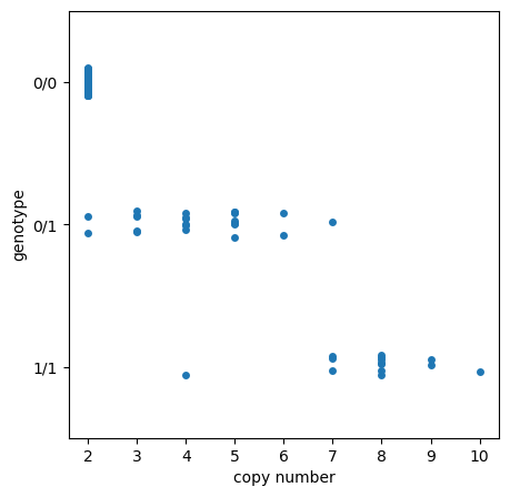
Calling SNPs at loci where there are CNVs is tricky, as the SNP calling model is expecting diploidy, but the CNV effectively makes an individual polyploid at that position. As we can see in the plot below, as copy number of Ace1 increases, it get’s less likely that the true heterozygote genotype is called.

Fortunately, the exact frequencies are not necessary, as being able to track the increase or decrease of these linked loci through time and space is what is important for informing insecticide use in vector control.

def genotype_by_copy_number(contig, position, sample_sets):
    import seaborn as sns
    import numpy as np
    import matplotlib.pyplot as plt
    geno = ag3.snp_genotypes(region=f"{contig}:{position}-{position+1}", sample_sets=sample_sets).compute()
    geno = geno[0]
    geno = np.apply_along_axis(arr=geno, func1d=lambda x: "/".join(map(str, x)), axis=1)

    ds_cnv = ag3.gene_cnv(region=f"{contig}:{position}-{position+1}", sample_sets=sample_sets)
    cnv_cn = ds_cnv['CN_mode'].compute().values[0]

    fig, ax = plt.subplots(1,1, figsize=[5,5])
    sns.stripplot(x=cnv_cn, y=geno, order = ['0/0','0/1','1/1'], ax=ax)
    plt.ylabel("genotype")
    plt.xlabel("copy number")
    plt.show()


genotype_by_copy_number(contig="2R", position=3492074, sample_sets="AG1000G-GH")

../_images/f11df8285e4d8bad5cd669d78354feadc21e8b46efc7f567199238d7d9d77364.png

What then now?#

Here we have demonstrated techniques that allow us to compare the frequency of SNPs and CNVs from the Ag3.0 data release together. However, the real power of these techniques to advance malaria control will come when they are applied to more recent data releases containing samples collected recently as spatial or temporal transects. With these data, associated SNPs and CNVs can be tracked together over space and time.

These analyses will need to be used in concert with others which are able to detect new loci under selection (see module 2 in this workshop). This is more relevant than ever with the large uptake in Actellic use (an organophosphate) for indoor residual spraying, as the established OP resistance mechanisms are likely to be supplemented by new loci and markers as mosquitoes evolve stronger resistance through greater exposure.

Practical exercise - Gste2#

English#

The Gste2 gene encodes an epsilon-class glutathione-S-transferase. It was initially studied in An. gambiae because its ortholog in the dengue and yellow fever vector Aedes aegypti has been linked to DDT resistance through increased gene expression.

One study looking at amino acid substitions in An. gambiae Gste2 found two mutations that in some cohorts were associated with insecticide resistance (Lucas et al. 2019). L119V was associated with permethrin (a type of pyrethroid) resistance and I114T was associated with both permethrin and DDT. Previously, Mitchell et al. (2014) found that Gste2 I114T conferred DDT resistance in An. gambiae and An. coluzzii.

The I114T mutation was also found to be associated with a CNV amplification that appeared to have fixed heterozygosity, much like with Ace1. The gene had duplicated, so that a wild-type gene and a I114T resistance mutation carrying gene were found on the same haplotype.

To further complicate the insecticide resistance story of Gste2 (and bring it into the scope of this module!) it has also been shown that overexpression of Gste2 is associated with OP resistance (Adolfi et al. 2019).

So, for this module’s practical excercise, I would like you run a case study on amino acid and CNV frequencies in Gste2, using the same analytical approach as we used for Ace1 and the An. coluzzii samples from Ag3.0.

1. Investigate amino acid frequencies in Gste2. HINT: transcript=”AGAP009194-RA”.

Why might the amino acid positional numbering go from high to low (opposite to Ace1)?

2. Examine CNVs in this region. HINT: region=”3R:28,597,652-28,598,640”

Plot a cnv_hmm_heatmap for the region - are there CNVs here?
Investigate gene cnv frequencies for Gste2.

3. Concatenate the amino acid frequency and gene cnv frequency DataFrames.

4. Visualise the concatenated DataFrame as heatmap. HINT: don’t forget to subset the DataFrame columns first.

Are there any clear patterns of association between SNP and CNV markers of insecticide resistance, like we found for Ace1? Why might this be the case?

5. If you would like to dig deeper into these analyses and their interpretations…

As an optional exercise, the Ace1 and Gste2 case studies could be repeated but looking at An. gambiae instead of An. coluzzii. HINT: remember the range of An. gambiae is larger than coluzzii.

Français#

Gste2 code pour une glutathion-S-transférase de classe epsilon. Il a été initialement étudié chez An. gambiae car son orthologue chez le vecteur de la dengue et de la fièvre jaune Aedes aegypti, a été connecté à une résistance au DDT par augmentation de l’expression génique.

Une étude observant les substitutions d’acides aminés chez An. gambiae pour Gste2 a trouvé deux mutations qui pour certaines cohortes étaient associées à une résistance aux insecticide (Lucas et al. 2019). L119V était associée à une résistance à la perméthrine (un type de pyrethrinoïde) et I114T était associée à une résistance à la fois à la perméthrine et au DDT. Précédemment, Mitchell et al. 2014 a montré que Gste2 I114T confère une résistance au DDT chez les An. gambiae et les An. coluzzii.

La mutation I114T était aussi associée à une amplification des CNVs, qui semble avoir une hétérozygotie fixée, de manière très similaire à Ace1. Ce gène était dupliquée, de telle sorte qu’un gène contenant l’allèle sauvage et un gène contenant I114T, l’allèle de résistance se trouvaient dans le même haplotype.

Pour compliquer encore l’histoire de la résistance aux insecticides liée à Gste2 (et la rapprocher du sujet de ce module!), il a aussi été montré que la surexpression de Gste2 est associée à une résistance aux OPs. (Adolfi et al. 2019).

Donc, pour l’exercice pratique de ce module, je voudrais que vous étudiez les fréquences des substitutions d’acides aminés et ses CNVs pour Gste2 en utilisant la même approche analytique que nous avons utilisée pour Ace1 et les échantillons de coluzzii d’Ag3.0.`

1. Etudier les fréquences des acides aminés pour Gste2. Indice: transcript=”AGAP009194-RA”.

Pourquoi est-ce que la numérotation des positions des acides aminés set décroissante (contrairement au cas d’Ace1)?

2. Examiner les CNVs dans cette région. Indice: region=”3R:28,597,652-28,598,640”

Afficher le diagramme cnv_hmm_heatmap pour cette région - quels CNVs sont présents?
Etudier les fréquences des CNVs pour Gste2.

3. Concaténer les DataFrames des fréquences des acides aminés et des fréquences des CNVs.

4. Visualiser le DataFrame obtenu par concaténation sous forme de heatmap. Indice: ne pas oublier de sélectionner les colonnes avant.

Y a-t-il des motifs clairs d’association enter les SNPs et les CNVs associés à la résistance aux insecticides, comme observé pour Ace1? Pourquoi cela?

5. Si vous souhaitez explorer ces analyses et leurs interprétations plus en profondeur…

En tant qu’exercice optionel, les études de cas pour Ace1 et Gste2 peuvent être répétées pour An. gambiae au lieu d’ An. coluzzii. Indice: se souvenir que la distribution des An. gambiae couvre une région plus vaste que celle des coluzzii.

Well done!#

In this module we have learnt how to:

Understand mechanisms and markers of organophosphate resistance.
Run amino acid frequency and CNV gene frequency analyses.
Combine and interpret SNP and CNV frequency data.

Exercises#

English#

Open this notebook in Google Colab and run it for yourself from top to bottom. As you run through the notebook, cell by cell, think about what each cell is doing, and try the practical exercises along the way.

Have go at the practical exercises, but please don’t worry if you don’t have time to do them all during the practical session, and please ask the teaching assistants for help if you are stuck.

Hint: To open the notebook in Google Colab, click the rocket icon at the top of the page, then select “Colab” from the drop-down menu.

Français#

Ouvrir ce notebook dans Google Colab et l’exécuter vous-même du début à la fin. Pendant que vous exécutez le notebook, cellule par cellule, pensez à ce que chaque cellule fait et essayez de faire les exercices quand vous les rencontrez.

Essayez de faire les exercices mais ne vous inquiétez pas si vous n’avez pas le temps de tout faire pendant la séance appliquée et n’hésitez pas à demander aux enseignants assistants si vous avez besoin d’aide parce que vous êtes bloqués.

Indice: Pour ouvrir le notebook dans Google Colab, cliquer sur l’icône de fusée au sommet de cette page puis choisissez “Colab” dans le menu déroulant.

Module 1 - Organophosphate resistance markers (combining SNP and CNV data)

Contents

Module 1 - Organophosphate resistance markers (combining SNP and CNV data)#

Learning Objectives#

Lecture#

English#

Français#

Setup#

Introduction#

The Ace1 gene#

Resistance to arganophosphate and carbamate insecticides#

Ace1 amino acid substitution frequencies#

Ace1 copy number variation frequencies#

Combining SNP and CNV allele frequencies#

What then now?#

Practical exercise - Gste2#

English#

Français#

Well done!#

Exercises#

English#

Français#