Module 1 - Interactive cloud computing with Google Colaboratory

Workshop 1 - Training course in data analysis for genomic surveillance of African malaria vectors

Module 1 - Interactive cloud computing with Google Colaboratory#

Theme: Tools & Technology

This first technology module introduces Google Colaboratory (a.k.a. Colab), an interactive cloud computing service for data analysis, which we will be using for practical exercises throughout the course.

Learning objectives#

After completing this module, you will be able to:

Explain what colab is
Explain what a notebook is
Access Colab and use it to create and run notebooks
Edit notebooks and create code and text cells
Be familiar with some basic coding in Python
Import and install packages
Share Colab notebooks via Google Drive

Lecture#

English#

Français#

Please note that the code in the cells below might differ from that shown in the video. This can happen because Python packages and their dependencies change due to updates, necessitating tweaks to the code.

What is Colab?#

Colab is an interactive cloud computing service provided for free by Google. To access Colab, visit the following address in your Web browser:

https://colab.research.google.com

To access Colab you will need a Google account. If you don’t already have one, create an account and then log in.

Colab allows you to write and execute code using your Web browser. There are two important features of Colab that are very useful for data analysis:

Interactive notebooks - You can explore and analyse data one step at a time, by writing small pieces of code, running them, inspecting the results, and then writing further code.
Cloud computing - You can get access to computers hosted by Google and use them to run your code, without having to install any software or download any data onto your own computer.

What is a notebook?#

A notebook is an interactive, editable document that you can use to:

Write and execute code
Create plots, tables, written text and other types of content

A notebook is built up from cells. There are two main types of cells in a notebook: code cells and text cells.

Code cells#

A code cell contains Python code. To add a code cell to your notebook, click the + Code button at the top of the notebook.

Below is an example code cell.

print("Hello world!")

Hello world!

Executing a code cell#

To execute a code cell, click on the play icon next to the cell. You can also type Shift+Enter, which will run the cell and move the focus to the next cell.

Cell output#

The code cell above uses the built-in print function, which prints the string "Hello world!" as output. If a code cell generates some output when it is run, the output is displayed below the cell.

Cells do not always have output. For example, the code cell below declares a variable named foo and assigns the integer value 42, but does not create an output.

foo = 42

Inspecting a variable#

If you have declared a variable, such as foo in the code cell above, and you want to inspect its value, you can do this by writing a code cell where the variable is written on the last line.

foo

Running this code cell will print the value of the variable as the cell output. Let’s try modifying this variable, and inspecting it again.

foo = foo + 1
foo

It can also sometimes be useful to use the built-in type() function inspect what type of object has been assigned to a variable, e.g.:

type(foo)

int

Text cells#

As well as code cells, you can also create text cells, which create text that you write, and can use different types of text formatting such as bold, italic, indented lists, hyperlinks and mathematical equations.

To add a text cell to your notebook, click the + Text button at the top of the notebook.

To edit an existing text cell in a notebook, double click on the cell.

Formatting text#

Text cells can be formatted using a special syntax called markdown.

Here is a quick summary of some useful markdown syntax for formatting text:

Markdown syntax	Preview
`bold text`	bold text
`italicized text`	italicized text
`monospace text`	`Monospace`
`[A link](https://en.wikipedia.org/wiki/Anopheles_gambiae)`	A link

Creating lists#

Unordered lists can be created by putting each list item on a new line, starting with the * character, e.g.:

* A list item
* Another list item
* Yet another list item

Ordered lists can be created by starting each list item with 1., e.g.:

First item
Second item
Third item

Creating section headings#

To create a section heading within a notebook, begin a line of text with the # character. E.g.:

# This is a section heading

To create a sub-section heading, begin a line of text with ##, E.g.:

## This is a sub-section heading

Adding images#

You can include an image in a notebook, if the image is published on the Web and you know it’s address. E.g., the markdown syntax below includes an image of an Anopheles gambiae mosquito available from wikipedia:

![Anopheles gambiae](https://upload.wikimedia.org/wikipedia/commons/0/0a/AnophelesGambiaemosquito.jpg)

Here is the image as it will appear in the notebook:

Anopheles gambiae

Adding, moving and deleting cells#

A new cell can be added by using the + Code and + Text at the top of the notebook, or that show when you hover between cells.

Cells can be moved within the notebook by clicking on the up and down arrows in the cell toolbar.

A cell can be deleted by clicking the dustbin icon within the cell toolbar.

Coding basics#

Here are a few examples of things you can do using Python code. For this course we don’t expect you to be an experienced coder, but some familiarity with features like arithmetic, for loops and functions will be useful.

Math#

You can do arithmetic.

x = 10
y = 3 + (4 * x) - 1
y

For loops#

You can use a for loop to iterate over a sequence of values. E.g., you can iterative over a sequence of numbers using a for loop together with the built-in range() function.

for i in range(5):
    print(i)

Defining and calling functions#

You can organise your code into functions with parameters. E.g., here we define a function greet() with a single parameter name.

def greet(name):
    print(f"Hello {name}!")

You can then call the function with different parameter values.

greet("Mario Coluzzi")

Hello Mario Coluzzi!

greet("Ronald Ross")

Hello Ronald Ross!

Importing and installing Python packages#

Python packages are collections of functions that other people have already created, and which you can import into your notebook and use.

There are some functions which are “built-in” to Python, like the print() and range() functions we’ve already seen, which are always available and you don’t need to import.

There are a lot more functions available as part of the Python standard library, which will already be installed, but you do need to import them before you can use them.

There are loads more functions available through “third-party packages” which are packages provided by other developers in the Python community. E.g., a very useful package for numerical computing is NumPy. On colab, numpy is already installed, and so you can just import it. By convention we abbreviate “numpy” to “np” just to reduce the amount of typing we have to do.

import numpy as np

Now that we’ve imported NumPy we can call functions. E.g., let’s generate some random numbers using the np.random.randint() function.

y = np.random.randint(low=0, high=100, size=10)
y

array([17, 23, 83, 74, 45, 81,  1, 21, 75, 99])

Some third-party packages are not pre-installed on colab, and so you need to install them. Installing packages can be done with the special !pip command. E.g., let’s installed the malariagen_data package.

%pip install -q --no-warn-conflicts malariagen_data

Once it’s installed, we can import it like we did for numpy.

import malariagen_data

And we can start using the package to set up access to some data.

ag3 = malariagen_data.Ag3()
ag3

MalariaGEN Ag3 API client
Please note that data are subject to terms of use, for more information see the MalariaGEN website or contact data@malariagen.net. See also the Ag3 API docs.
Storage URL	gs://vo_agam_release/
Data releases available	3.0, 3.1, 3.2, 3.3, 3.4, 3.5, 3.6, 3.7, 3.8
Results cache	None
Cohorts analysis	20231215
AIM analysis	20220528
Site filters analysis	dt_20200416
Software version	malariagen_data 8.7.0
Client location	unknown

Viewing dataframes#

Often when analysing data you will work with pandas DataFrames, which are tables of data organised into rows and columns. We will look at DataFrames in more detail later in the course, but for now it’s useful to know that you can get a preview of the data in a DataFrame.

E.g., if we call the sample_metadata() function below, this returns a DataFrame.

df_samples = ag3.sample_metadata(sample_sets="3.0")

type(df_samples)

pandas.core.frame.DataFrame

If we now inspect the value of this variable, we get a preview of the data in the DataFrame, showing the first five rows and the last five rows.

df_samples

	sample_id	partner_sample_id	contributor	country	location	year	month	latitude	longitude	sex_call	...	admin1_name	admin1_iso	admin2_name	taxon	cohort_admin1_year	cohort_admin1_month	cohort_admin1_quarter	cohort_admin2_year	cohort_admin2_month	cohort_admin2_quarter
0	AR0047-C	LUA047	Joao Pinto	Angola	Luanda	2009	4	-8.884	13.302	F	...	Luanda	AO-LUA	Luanda	coluzzii	AO-LUA_colu_2009	AO-LUA_colu_2009_04	AO-LUA_colu_2009_Q2	AO-LUA_Luanda_colu_2009	AO-LUA_Luanda_colu_2009_04	AO-LUA_Luanda_colu_2009_Q2
1	AR0049-C	LUA049	Joao Pinto	Angola	Luanda	2009	4	-8.884	13.302	F	...	Luanda	AO-LUA	Luanda	coluzzii	AO-LUA_colu_2009	AO-LUA_colu_2009_04	AO-LUA_colu_2009_Q2	AO-LUA_Luanda_colu_2009	AO-LUA_Luanda_colu_2009_04	AO-LUA_Luanda_colu_2009_Q2
2	AR0051-C	LUA051	Joao Pinto	Angola	Luanda	2009	4	-8.884	13.302	F	...	Luanda	AO-LUA	Luanda	coluzzii	AO-LUA_colu_2009	AO-LUA_colu_2009_04	AO-LUA_colu_2009_Q2	AO-LUA_Luanda_colu_2009	AO-LUA_Luanda_colu_2009_04	AO-LUA_Luanda_colu_2009_Q2
3	AR0061-C	LUA061	Joao Pinto	Angola	Luanda	2009	4	-8.884	13.302	F	...	Luanda	AO-LUA	Luanda	coluzzii	AO-LUA_colu_2009	AO-LUA_colu_2009_04	AO-LUA_colu_2009_Q2	AO-LUA_Luanda_colu_2009	AO-LUA_Luanda_colu_2009_04	AO-LUA_Luanda_colu_2009_Q2
4	AR0078-C	LUA078	Joao Pinto	Angola	Luanda	2009	4	-8.884	13.302	F	...	Luanda	AO-LUA	Luanda	coluzzii	AO-LUA_colu_2009	AO-LUA_colu_2009_04	AO-LUA_colu_2009_Q2	AO-LUA_Luanda_colu_2009	AO-LUA_Luanda_colu_2009_04	AO-LUA_Luanda_colu_2009_Q2
...	...	...	...	...	...	...	...	...	...	...	...	...	...	...	...	...	...	...	...	...	...
3076	AD0494-C	80-2-o-16	Martin Donnelly	Lab Cross	LSTM	-1	-1	53.409	-2.969	F	...	NaN	NaN	NaN	unassigned	NaN	NaN	NaN	NaN	NaN	NaN
3077	AD0495-C	80-2-o-17	Martin Donnelly	Lab Cross	LSTM	-1	-1	53.409	-2.969	M	...	NaN	NaN	NaN	unassigned	NaN	NaN	NaN	NaN	NaN	NaN
3078	AD0496-C	80-2-o-18	Martin Donnelly	Lab Cross	LSTM	-1	-1	53.409	-2.969	M	...	NaN	NaN	NaN	unassigned	NaN	NaN	NaN	NaN	NaN	NaN
3079	AD0497-C	80-2-o-19	Martin Donnelly	Lab Cross	LSTM	-1	-1	53.409	-2.969	F	...	NaN	NaN	NaN	unassigned	NaN	NaN	NaN	NaN	NaN	NaN
3080	AD0498-C	80-2-o-20	Martin Donnelly	Lab Cross	LSTM	-1	-1	53.409	-2.969	M	...	NaN	NaN	NaN	unassigned	NaN	NaN	NaN	NaN	NaN	NaN

3081 rows × 32 columns

Creating plots#

You can also create plots within notebooks. There are several plotting packages available for Python, but three popular and useful plotting packages are matplotlib, plotly express, and bokeh. Let’s illustrate making some plots with these packages.

First let’s generate some random data to plot.

x = np.random.binomial(n=30, p=0.5, size=10_000)
x

array([12, 18, 16, ..., 20, 18, 14])

Matplotlib#

Here’s how to import and activate matplotlib in a notebook.

import matplotlib.pyplot as plt
%matplotlib inline

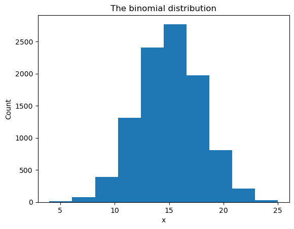
Here’s how to create a histogram.

fig, ax = plt.subplots()
ax.hist(x)
ax.set_xlabel("x")
ax.set_ylabel("Count")
ax.set_title("The binomial distribution");

../_images/c375a26600c8f5ed74e38260c56b400d7edbf431048435de3b3898cc7e9ebdb1.png

Plotly Express#

Here’s how to import plotly express.

import plotly.express as px

Here’s how to plot a histogram.

fig = px.histogram(
    x=x, 
    title="The binomial distribution",
    width=600,
    height=400
)

fig.show()

Bokeh#

Here’s how to import bokeh and activate it for use in a notebook.

import bokeh.plotting as bkplt
import bokeh.io as bkio
bkio.output_notebook()

Loading BokehJS ...

Here’s how to make a histogram.

fig = bkplt.figure(title="The binomial distribution", width=600, height=400)
hist, edges = np.histogram(x)
fig.quad(top=hist, bottom=0, left=edges[:-1], right=edges[1:])
bkplt.show(fig)

Accessing help documentation (docstrings)#

Often you’ll want to get access to documentation about the packages and functions you’re using. An easy way to access documentation (the docstring) for a function is to type the function name then add a question mark (?). This will cause the docstring to appear next to the notebook.

np.random.binomial?

You can also search the web. Most packages will have good documentation on their website. E.g., here’s the online documentation for np.random.binomial().

Practical exercises#

English#

That’s it for this module, well done for beginning your data analysis journey! When you’re ready, please now try the practical exercises below.

Go to https://colab.research.google.com and create a new notebook.
Add a code cell, type some Python code, and run (execute) the cell.
Add a text cell and type some text, using markdown to format the text, e.g., bold, italic, hyperlinks, etc.
Practice adding, deleting and moving cells within the notebook.
Import a package (e.g., numpy) and call a function from that package (e.g., numpy.random.randint()). Hint: use ? to display the function parameters if you can’t remember them.
Add a code cell which creates a pandas DataFrame. Hint: you can search the web for pandas code examples, and copy-paste the code into your notebook.
Add a code cell which creates a matplotlib plot. Hint: try the matplotlib examples gallery for some code examples to try.
Add a code cell which creates a plotly plot. Hint: try the plotly express docs for some code examples to try.
Add a code cell which creates a bokeh plot. Hint: try the bokeh gallery for some code examples to try.

Français#

C’est tout pour ce module, félicitations pour le début de votre voyage dans le monde de l’analyse des données! Quand vous êtes prêts, essayez les exercices appliqués ci-dessous.

Se rendre sur https://colab.research.google.com et créer un nouveau notebook.
Créer une nouvelle cellule de code, entrer du code Python et exécuter la cellule.
Ajouter une cellule de texte et entrer du texte, utiliser le markdown pour modifier son format, par exemple en mettant en gras ou en italique certains mots ou en ajoutant un hyperlien.
S’entrainer à ajouter, supprimer et déplacer les cellules.
Importer un paquet (par exemple, numpy) et utiliser une fonction de ce paquet (par exemple, numpy.random.randint()). Indice: utiliser ? pour afficher les paramètres si vous les avez oubliés.
Ajouter une cellule de code qui crée un DataFrame pandas. Indice: vous pouvez chercher un exemple de code pour pandas sur internet et copier-coller le code dans votre notebook.
Ajouter une cellule de code qui crée un graphe matplotlib. Indice: essayer la gallerie d’exemples matplotlib pour des exemples de code.
Ajouter une cellule de code qui crée un graphe plotly. Indice essayer les docs plotly express pour des exemples de code.
Ajouter une cellule de code qui crée un graphe bokeh. Indice: essayer la gallerie bokeh pour des exemples de code.

Module 1 - Interactive cloud computing with Google Colaboratory

Contents

Module 1 - Interactive cloud computing with Google Colaboratory#

Learning objectives#

Lecture#

English#

Français#

What is Colab?#

What is a notebook?#

Code cells#

Executing a code cell#

Cell output#

Inspecting a variable#

Text cells#

Formatting text#

Creating lists#

Creating section headings#

Adding images#

Adding, moving and deleting cells#

Coding basics#

Math#

For loops#

Defining and calling functions#

Importing and installing Python packages#

Viewing dataframes#

Creating plots#

Matplotlib#

Plotly Express#

Bokeh#

Accessing help documentation (docstrings)#

Sharing notebooks via Google Drive#

Practical exercises#

English#

Français#